|
|
|
|
|
|
| |
| |
|
|
|
|
| |
| |
|
|
What I forgot: I turned on radiosity as yoou mentioned but without a light
source the image was black, except for the emitters (if using a black
background). Why is that?
I think I now got what most of you meant. In my words ... suppose I have the
field data (say intensity) in a CSV file. Let's say I read that file in and
generate an array from it:
#declare N_points_in_file = 1000;
#declare Field_values = array[N_points_in_file];
#declare Index = 0;
#fopen MyFile "field_filename.csv" read
#while (defined(MyFile))
#read (MyFile, X, Y, Z, Field_intensity)
#declare Field_values[Index] = <X, Y, Z, Intensity>;
#declare Index = Index + 1;
#end
Now the array `Field_values` holds all the points and the respective
intensities. Next, I would define an object of the size of my volume, i.e.
a union of the cylinder filling up the hole and another hexahedron above the
structure. Suppose this object is defined as `Field_volume`, I than would have
to set the interior like this
interior
{ media
{ emission Intensity
density {
function { ... Field_value_interpolated(x,y,z) ... }
color_map {
... "My color map definition" ...
}
}
}
}
here, `Field_value_interpolated` has to be a function that connects the x,y,z
coordinate to the `Field_intensity` in the `Field_values` array given above.
But for this I would have to find the closest coordinate in the array, right?
Or even use an interpolator?
Moreover, what are the x,y,z that the density function passes?
Post a reply to this message
|
|
| |
| |
|
|
|
|
| |
| |
|
|
"cbpypov" <nomail@nomail> wrote:
> What I forgot: I turned on radiosity as yoou mentioned but without a light
> source the image was black, except for the emitters (if using a black
> background). Why is that?
>
> I think I now got what most of you meant. In my words ... suppose I have the
> field data (say intensity) in a CSV file. Let's say I read that file in and
> generate an array from it:
>
> #declare N_points_in_file = 1000;
> #declare Field_values = array[N_points_in_file];
> #declare Index = 0;
> #fopen MyFile "field_filename.csv" read
> #while (defined(MyFile))
> #read (MyFile, X, Y, Z, Field_intensity)
> #declare Field_values[Index] = <X, Y, Z, Intensity>;
> #declare Index = Index + 1;
> #end
>
> Now the array `Field_values` holds all the points and the respective
> intensities. Next, I would define an object of the size of my volume, i.e.
> a union of the cylinder filling up the hole and another hexahedron above the
> structure. Suppose this object is defined as `Field_volume`, I than would have
> to set the interior like this
>
> interior
> { media
> { emission Intensity
> density {
> function { ... Field_value_interpolated(x,y,z) ... }
> color_map {
> ... "My color map definition" ...
> }
> }
>
> }
> }
>
> here, `Field_value_interpolated` has to be a function that connects the x,y,z
> coordinate to the `Field_intensity` in the `Field_values` array given above.
> But for this I would have to find the closest coordinate in the array, right?
> Or even use an interpolator?
>
> Moreover, what are the x,y,z that the density function passes?
So I finally arrived at the point discussed above. See the file attached which
includes a very coarse field for testing. It contains 5 columns, say: index, x,
y, z, intensity. The x,y,z coordinates are in nm, i.e. must be divided by a_real
in my code. Moreover, I did not manage yet to export the field in _only_ the
volume where I want to show it. The z-coordinate must therefore be shifted by
-250. to align the field with the pov coordinates. I normalized the intensity
column to range from 0. to 1.
I am reading the file as follows, which seems to work out fine:
// Reading the field distribution file
//--------------------------------------------------------------------------
#declare N_points_in_file = 4608;
#declare Field_values = array[N_points_in_file];
#declare Index = 0;
#fopen MyFile "field_coarse_correct.csv" read
#while (defined(MyFile))
#read (MyFile, FIndex, X, Y, Z, Field_intensity)
#declare Field_values[Index] = <X/a_real, Y/a_real, (Z-250.)/a_real,
Field_intensity>;
#declare Index = Index + 1;
#end
Now I thought I could just define the density mapping using this array!?
However, the docs
http://www.povray.org/documentation/3.7.0/r3_4.html#r3_4_8_4_3
say something abount density lists, but more or less only this rather cryptic
sentence:
"You may declare and use density map identifiers but the only way to declare a
density block pattern list is to declare a density identifier for the entire
density."
I appreciate any code examples on how to get beyond the point I am at now :)
Post a reply to this message
Attachments:
Download 'field_coarse_correct.csv.txt' (221 KB)
|
|
| |
| |
|
|
|
|
| |
| |
|
|
"cbpypov" <nomail@nomail> wrote:
> What I forgot: I turned on radiosity as yoou mentioned but without a light
> source the image was black, except for the emitters (if using a black
> background). Why is that?
Because those are the only things that emit any light. If you need a light
source, then define a thing - a light panel (box{}) a tube (cylinder{}) a CSG
lightbulb, etc. that has an emission value. The stronger the emission, the more
light. You may need to define diffuse or specular in a finish block for your
other objects to reflect light back to the camera and make them more visible.
Let's say I read that file in and
> generate an array from it:
.....
> Now the array `Field_values` holds all the points and the respective
> intensities.
.....
>
> here, `Field_value_interpolated` has to be a function that connects the x,y,z
> coordinate to the `Field_intensity` in the `Field_values` array given above.
Well, you're kinda going around in a circle - if you have _data_ then you should
use that to create a df3 file - voxels. IIRC POV-Ray has different ways of
interpolating based on those (trilinear, tricubic, etc.)
> Moreover, what are the x,y,z that the density function passes?
POV-Ray will evaluate your density "function" based on all of the x, y, and z
coordinates in the unit cube that the media occupies.
See my re-invention of POV-Ray's isosurface "wheel":
http://news.povray.org/povray.binaries.images/thread/%3Cweb.59cf0d20e6e56be5cafe28e0%40news.povray.org%3E/
Most notably the x, y, z nested loops at the end of the code.
My idea was that if you were generating the data in your CSV file with an
equation, then you could bypass all that and just use that equation as your
density function directly. But I don't know all of the details of how you're
putting this together - I have no "bigger picture" yet.
Post a reply to this message
|
|
| |
| |
|
|
|
|
| |
| |
|
|
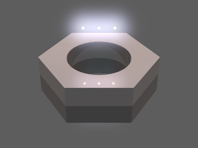
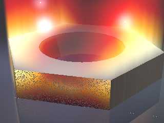
So, this is what I have using what I've managed to assemble from your code so
far:
I set absorption to 0 - because you want pure emission, not any absorption of
one glow to absorb the emission from another.
Post a reply to this message
Attachments:
Download 'quantumdot0.png' (44 KB)
Preview of image 'quantumdot0.png'
|
|
| |
| |
|
|
|
|
| |
| |
|
|
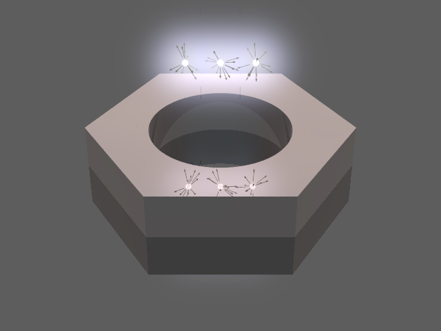
And just some random arrows using VRand_On_Sphere () before I hit the sack.
#declare Rad = 0.0125;
#declare Intense = 0.5;
#declare Rays = 12;
#declare Stream = seed (123);
#declare Line = 0.00125;
#declare Glow = 20;
#macro GlowRays ()
union{
#for (R, 1, Rays)
#declare Start = VRand_On_Sphere (Stream)*Rad*2;
#declare End = Start*Glow/6;
object {Vector (Start, End, Line) texture {pigment {Yellow} finish {diffuse
1}}}
#end
no_shadow
}
#end
#for (X, -1, 1)
QuantumDot (Rad, Rad*Glow, Intense, <X/7, 0.5, 0>)
object {GlowRays () translate <X/7, 0.5, 0>}
#end
I think now is the time to get an overall idea of your final render, so you can
structure things to best accomplish that, rather than let this thing get too
"organically-grown" and hard to re-write.
Post a reply to this message
Attachments:
Download 'quantumdot0.png' (52 KB)
Preview of image 'quantumdot0.png'
|
|
| |
| |
|
|
|
|
| |
| |
|
|
"Bald Eagle" <cre### [at] netscape net> wrote:
> And just some random arrows using VRand_On_Sphere () before I hit the sack.
>
> #declare Rad = 0.0125;
> #declare Intense = 0.5;
> #declare Rays = 12;
> #declare Stream = seed (123);
> #declare Line = 0.00125;
> #declare Glow = 20;
>
> #macro GlowRays ()
> union{
> #for (R, 1, Rays)
> #declare Start = VRand_On_Sphere (Stream)*Rad*2;
> #declare End = Start*Glow/6;
> object {Vector (Start, End, Line) texture {pigment {Yellow} finish {diffuse
> 1}}}
> #end
> no_shadow
> }
> #end
>
> #for (X, -1, 1)
> QuantumDot (Rad, Rad*Glow, Intense, <X/7, 0.5, 0>)
> object {GlowRays () translate <X/7, 0.5, 0>}
> #end
>
>
> I think now is the time to get an overall idea of your final render, so you can
> structure things to best accomplish that, rather than let this thing get too
> "organically-grown" and hard to re-write.
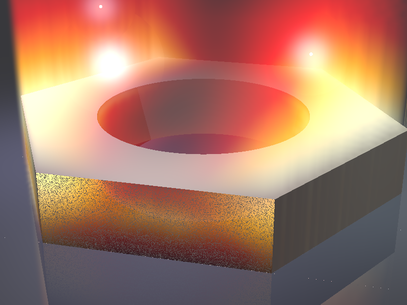
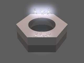
Hello everyone. So you convinced me and I chose the df3 route which turns out to
work absolutely well. I used the python df3 library you had linked and created
one file for each component of RGB using the colormap I like. For the media
settings I was using Stephens code (thank you very much! A small thing: the
`hollow` keyword was missing :) ).
I further set the QD absorption to 0. as Bald Eagle suggested. I really like the
arrow thing you posted, but somehow I could not figure out where the `Vector`
function comes from? My povray does not know it and I could not find an .inc
that defines it. Could you post more code that you used for the image with
arrows? I'll attach an image of the single unit cell here, together with 3
example quantum dots.
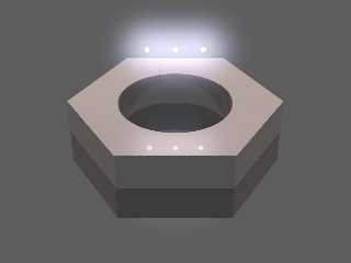
In the next to posts I will attach an image of the _patterned_ version, which is
not working yet because the boxes in which the field is defined overlap. How can
I solve this problem?
Basically, I think it is almost done and I thank you all so very much. A few
final things remain:
- The emitters: is it possible to choose some random coordinates in each
unit cell and read the emitter intensity from the df3 file as well?
(the intensity of the emitters should correspond to the field intensity
at their positions)
- Making a _great_ render of this nice approach :) Maybe this is to much to
ask for, but I think the really important thing is to tune the materials,
lights and quality options to gain a really stunning image in the end.
Unfortunately I do not seem to have enough overview of these things. Is
it possible that you would help me with it?
Finally, I cleaned up the code. Here it is:
//
// Author: Carlo Barth
// Date: 2016/10/21
//
// Purpose: A high-quality, artistic render of quantum dots (QDs) near a
// photonic crystal surface, interacting with a leaky-mode.
// The leaky mode is represented by a color-coded volume render.
// The QDs have an emission proportional to the local field energy
// density, denoted by a glowing aura and random arrows.
//
// Details: The data is based on a finite element method solve of the
// photonic crystal on glass. The glass substrate is omitted in the
// render. See the related paper describing most of the experimental
// and numerical methods and results:
//
// http://aip.scitation.org/doi/10.1063/1.4995229
//
// Imports
//--------------------------------------------------------------------------
#include "colors.inc"
#include "textures.inc"
#include "glass.inc"
#include "metals.inc"
#include "rand.inc"
//==========================================================================
// SECTION: Parameters and settings
//==========================================================================
// Global Settings
//--------------------------------------------------------------------------
#version 3.7;
global_settings{
assumed_gamma 1.0
}
// Global parameters
//--------------------------------------------------------------------------
// 0=off, 1=fast; 2=medium quality; 3=high qual.;
// 4= medium qual.+ recursion_limit 2
#declare Radiosity_On = 0;
#declare Spot_on = true; // whether to use spot lights
#declare Camera_Type = 2; // 1 = wide view, 2 = close-up
// Real geometry parameters in nanometer
#declare a_real = 600.; // lattice constant
#declare d_real = 367.; // hole diameter
#declare h_real = 116.; // phc height
#declare r_qds_real = 2.8; // radius quantum dots (QD)
#declare r_qds_aura = 15; // maximum radius factor for QD aura
// extent of the field volume
#declare field_box_dim_real = <692.820, 610., 600.>;
// translation vector for field volume alignment
#declare field_box_trans_real = <-346.41016151400004, -250., -300.>;
// Derived parameters and abbreviating expressions
#declare a = a_real/a_real;
#declare d = d_real/a_real;
#declare h = h_real/a_real;
#declare r_qds = r_qds_real/a_real;
#declare field_box_dim = field_box_dim_real/a_real;
#declare field_box_trans = field_box_trans_real/a_real;
#declare sqrt3 = 0.5*sqrt(3.); // for hexagonal lattice
#declare cx = a/sqrt3/4; // standard x coordinate of hexagon
#declare cy = 0.5*a; // standard y coordinate of hexagon
#declare Repeat_unit_cells = false; // whether to repeat the unit cell
#declare rows = 5; // rows of the unit cell repetition pattern
#declare cols = 5; // columns of the unit cell repetition pattern
// Parameters related to artistic depections, rather than real properties
#declare r_aura = r_qds*r_qds_aura; // radius QD aura max (in diameters)
#declare Field_brightness = 3.; // Brightness of the field render
#declare Field_interpolation = 1; // Brightness of the field render
// Camera
//--------------------------------------------------------------------------
#switch (Camera_Type)
#case (1)
#declare Camera = camera {
angle 40
location <0, 2, -3>
look_at <0, h/2, 0>
right x*image_width/image_height
}
#break
#case (2)
#declare Camera = camera {
angle 30
location <0.5, h*5, -2>
look_at <0, h/3, 0>
right x*image_width/image_height
}
#break
#end // end of switch
camera{Camera}
//==========================================================================
// SECTION: Illumination
//==========================================================================
// Radiosity
//--------------------------------------------------------------------------
#if (Radiosity_On > 0)
global_settings {
#ifndef ( Rad_Quality )
#declare Rad_Quality = Radiosity_On;
#end
//--------- radiosity settings -------------------------------- ///
// from POV-Ray samples "scene templates/patio-radio.pov
#switch (Rad_Quality)
#case (1)
radiosity { // --- Settings 1 (fast) ---
pretrace_start 0.08
pretrace_end 0.02
count 50
error_bound 0.5
recursion_limit 1
}
#break
#case (2)
radiosity { // --- Settings 2 (medium quality) ---
pretrace_start 0.08
pretrace_end 0.01
count 120
error_bound 0.25
recursion_limit 1
}
#break
#case (3)
radiosity { // --- Settings 3 (high quality) ---
pretrace_start 0.08
pretrace_end 0.005
count 400
error_bound 0.1
recursion_limit 1
}
#break
#case (4)
radiosity { // --- Settings 4 (medium quality, recursion_limit)
pretrace_start 0.08
pretrace_end 0.005
count 350
error_bound 0.15
recursion_limit 2
}
#break
#case (5)
radiosity { // --- Settings 5 (high quality, recursion_limit )
pretrace_start 0.08
pretrace_end 0.005
count 350
error_bound 0.1
recursion_limit 2
}
#break
#end // end of switch
} // end of global settings
#default{ finish {emission 0. diffuse 0. ambient 0.}}
//--------------------------------------------------------------------------
#else
#default{ finish{ ambient 0.1 diffuse 0.9 }
} // for intel computers
#end
// Light sources
//--------------------------------------------------------------------------
// A group of 3 spot lights
#if (Spot_on)
light_source{ // greenish
<1.,15*h,-1> color rgb <.8,1,.8>
spotlight
point_at<0.5,0,0>
radius 60 // hotspot
tightness 100
falloff 90
}
light_source{ // blueish
<-1.,15*h,-1> color rgb <.8,.8,1>
spotlight
point_at<-0.5,0,0>
radius 60 // hotspot
tightness 100
falloff 90
}
light_source{ // "white"
<0,15*h,-1> color rgb <.8,.8,.8>
spotlight
point_at<0.,0,-0.5>
radius 60 // hotspot
tightness 100
falloff 90
}
#end
//==========================================================================
// SECTION: Object description
//==========================================================================
// Textures
//--------------------------------------------------------------------------
// Material of the photonic crystal
#declare t_shiny_metal =
texture {
pigment {
rgb <.55, .42, .41>
}
finish {
specular 0.2 roughness 0.5
brilliance 4
}
}
// Functions
//--------------------------------------------------------------------------
// Spherical exponential decay
#declare Exp_decay = function (x, y, z, Rad_factor) {
exp( -(pow(x,2) + pow(y,2) + pow(z,2))*60/Rad_factor )
};
// Macros
//--------------------------------------------------------------------------
// The quantum dot macro
#macro QuantumDot(Radius, Radius_aura, Intensity, Origin)
// The actual quantum dot
sphere{
<0,0,0>, Radius
texture{ Glass2 } // end of texture
translate Origin
} // end of sphere
// The glowing aura
sphere {
<0,0,0>,
Radius_aura*(1+Intensity) //Radius* (Intensity*r_qds_aura + 1)
pigment { rgbt 1 } hollow
interior
{ media
{ emission Intensity*10
density {
function { Exp_decay(x, y, z, Radius_aura*(1+Intensity)) }
color_map {
[0.0 rgbt <0,0,0,0>]
[0.5 rgbt <0.5, 0.5, 0.7,0>]
[1.0 rgbt <1,1,1,0>]
}
}
}
media
{ absorption 0.
}
}
translate Origin
}
// #end // end of #for loop
#end // ------------------ end of macro
// Loop for triangular lattice
//--------------------------------------------------------------------------
#macro TriangularLoop ( Object, trans_vec )
#local ii = -cols;
#while ( ii < cols )
#local jj = -rows;
#while ( jj < rows )
#if ( mod(ii,2) = 0 )
#local hexshift = 0.5*a;
#else
#local hexshift = 0.;
#end
object{
Object
translate <ii*a*sqrt3, 0., jj*a+hexshift>
translate trans_vec
}
#local jj = jj+1;
#end
#local ii = ii+1;
#end
#end // ------------------ end of macro
// Compound objects
//--------------------------------------------------------------------------
// Silicon material in the hexagonal unit cell
#declare geo_si = prism {
linear_sweep
linear_spline
0., // sweep the following shape from here ...
h, // ... up through here
7, // the number of points making up the shape ...
<-2*cx,0>, <-cx,cy>, <cx,cy>, <2*cx,0>, <cx,-cy>, <-cx,-cy>, <-2*cx,0>
}
// Cylinder representing the hole in the silicon
#declare geo_hole = cylinder {
<0., -0.1, 0.>, <0., h+0.1, 0.>, d/2.
}
// Photonic crystal in unit cell by difference of silicon membrane and hole
#declare phc = difference {
object{ geo_si }
object{ geo_hole }
}
// A single unit cell of the photonic crystal
//--------------------------------------------------------------------------
#declare PhC_object = object{
phc
texture{ t_shiny_metal }
}
// Field render in unit cell
//--------------------------------------------------------------------------
#declare Field_object = box {
<0,0,0>, <1,1,1>
texture {
pigment {
colour rgbft <1.000,1.000,1.00,0.000,1.000>
}
}
hollow
interior{
ior 1.000
caustics 0.000
dispersion 1.000
dispersion_samples 7.000
fade_power 0.000
fade_distance 0.000
fade_color rgb <0.000,0.000,0.000>
// Red
media {
method 3
intervals 10
samples 1, 1
confidence 0.900
variance 0.008
ratio 0.900
absorption rgb <0,0,0>
emission rgb <1,0,0> * Field_brightness
aa_threshold 0.050
aa_level 4
density {
density_file df3 "efield_energy_in_superspace_R.df3"
interpolate Field_interpolation
}
}
// Green
media {
method 3
intervals 10
samples 1, 1
confidence 0.900
variance 0.008
ratio 0.900
absorption rgb <0,0,0>
emission rgb <0,1,0> * Field_brightness
aa_threshold 0.050
aa_level 4
density {
density_file df3 "efield_energy_in_superspace_G.df3"
interpolate Field_interpolation
}
}
// Blue
media {
method 3
intervals 10
samples 1, 1
confidence 0.900
variance 0.008
ratio 0.900
absorption rgb <0,0,0>
emission rgb <0,0,1> * Field_brightness
aa_threshold 0.050
aa_level 4
density {
density_file df3 "efield_energy_in_superspace_B.df3"
interpolate Field_interpolation
}
}
}
// Set proper size and position
scale field_box_dim
translate field_box_trans
}
// Union of PhC and field
#declare PhC_with_Field = union {
object{ PhC_object }
object{ Field_object }
}
//==========================================================================
// SECTION: Objects in scene
//==========================================================================
// Background
background{White*0.6}
// Floor
//--------------------------------------------------------------------------
plane
{ y, 0.
material{
texture {
pigment{ rgb<.1,.1,.15>}
finish {
reflection .05
}
}
}
}
// Photonic crystal with field render
#if (Repeat_unit_cells)
union{
TriangularLoop ( PhC_with_Field, <0,0,0> )
}
#else
PhC_with_Field
#end
// Some quantum dots
QuantumDot( r_qds, r_aura, 0.6, <0.3, 2*h, 0.>)
QuantumDot( r_qds, r_aura, 0.4, <-0.3, 2.5*h, 0.>)
QuantumDot( r_qds, r_aura, 1.0, <-0.2, 2*h, -0.2>) net> wrote:
> And just some random arrows using VRand_On_Sphere () before I hit the sack.
>
> #declare Rad = 0.0125;
> #declare Intense = 0.5;
> #declare Rays = 12;
> #declare Stream = seed (123);
> #declare Line = 0.00125;
> #declare Glow = 20;
>
> #macro GlowRays ()
> union{
> #for (R, 1, Rays)
> #declare Start = VRand_On_Sphere (Stream)*Rad*2;
> #declare End = Start*Glow/6;
> object {Vector (Start, End, Line) texture {pigment {Yellow} finish {diffuse
> 1}}}
> #end
> no_shadow
> }
> #end
>
> #for (X, -1, 1)
> QuantumDot (Rad, Rad*Glow, Intense, <X/7, 0.5, 0>)
> object {GlowRays () translate <X/7, 0.5, 0>}
> #end
>
>
> I think now is the time to get an overall idea of your final render, so you can
> structure things to best accomplish that, rather than let this thing get too
> "organically-grown" and hard to re-write.
Hello everyone. So you convinced me and I chose the df3 route which turns out to
work absolutely well. I used the python df3 library you had linked and created
one file for each component of RGB using the colormap I like. For the media
settings I was using Stephens code (thank you very much! A small thing: the
`hollow` keyword was missing :) ).
I further set the QD absorption to 0. as Bald Eagle suggested. I really like the
arrow thing you posted, but somehow I could not figure out where the `Vector`
function comes from? My povray does not know it and I could not find an .inc
that defines it. Could you post more code that you used for the image with
arrows? I'll attach an image of the single unit cell here, together with 3
example quantum dots.
In the next to posts I will attach an image of the _patterned_ version, which is
not working yet because the boxes in which the field is defined overlap. How can
I solve this problem?
Basically, I think it is almost done and I thank you all so very much. A few
final things remain:
- The emitters: is it possible to choose some random coordinates in each
unit cell and read the emitter intensity from the df3 file as well?
(the intensity of the emitters should correspond to the field intensity
at their positions)
- Making a _great_ render of this nice approach :) Maybe this is to much to
ask for, but I think the really important thing is to tune the materials,
lights and quality options to gain a really stunning image in the end.
Unfortunately I do not seem to have enough overview of these things. Is
it possible that you would help me with it?
Finally, I cleaned up the code. Here it is:
//
// Author: Carlo Barth
// Date: 2016/10/21
//
// Purpose: A high-quality, artistic render of quantum dots (QDs) near a
// photonic crystal surface, interacting with a leaky-mode.
// The leaky mode is represented by a color-coded volume render.
// The QDs have an emission proportional to the local field energy
// density, denoted by a glowing aura and random arrows.
//
// Details: The data is based on a finite element method solve of the
// photonic crystal on glass. The glass substrate is omitted in the
// render. See the related paper describing most of the experimental
// and numerical methods and results:
//
// http://aip.scitation.org/doi/10.1063/1.4995229
//
// Imports
//--------------------------------------------------------------------------
#include "colors.inc"
#include "textures.inc"
#include "glass.inc"
#include "metals.inc"
#include "rand.inc"
//==========================================================================
// SECTION: Parameters and settings
//==========================================================================
// Global Settings
//--------------------------------------------------------------------------
#version 3.7;
global_settings{
assumed_gamma 1.0
}
// Global parameters
//--------------------------------------------------------------------------
// 0=off, 1=fast; 2=medium quality; 3=high qual.;
// 4= medium qual.+ recursion_limit 2
#declare Radiosity_On = 0;
#declare Spot_on = true; // whether to use spot lights
#declare Camera_Type = 2; // 1 = wide view, 2 = close-up
// Real geometry parameters in nanometer
#declare a_real = 600.; // lattice constant
#declare d_real = 367.; // hole diameter
#declare h_real = 116.; // phc height
#declare r_qds_real = 2.8; // radius quantum dots (QD)
#declare r_qds_aura = 15; // maximum radius factor for QD aura
// extent of the field volume
#declare field_box_dim_real = <692.820, 610., 600.>;
// translation vector for field volume alignment
#declare field_box_trans_real = <-346.41016151400004, -250., -300.>;
// Derived parameters and abbreviating expressions
#declare a = a_real/a_real;
#declare d = d_real/a_real;
#declare h = h_real/a_real;
#declare r_qds = r_qds_real/a_real;
#declare field_box_dim = field_box_dim_real/a_real;
#declare field_box_trans = field_box_trans_real/a_real;
#declare sqrt3 = 0.5*sqrt(3.); // for hexagonal lattice
#declare cx = a/sqrt3/4; // standard x coordinate of hexagon
#declare cy = 0.5*a; // standard y coordinate of hexagon
#declare Repeat_unit_cells = false; // whether to repeat the unit cell
#declare rows = 5; // rows of the unit cell repetition pattern
#declare cols = 5; // columns of the unit cell repetition pattern
// Parameters related to artistic depections, rather than real properties
#declare r_aura = r_qds*r_qds_aura; // radius QD aura max (in diameters)
#declare Field_brightness = 3.; // Brightness of the field render
#declare Field_interpolation = 1; // Brightness of the field render
// Camera
//--------------------------------------------------------------------------
#switch (Camera_Type)
#case (1)
#declare Camera = camera {
angle 40
location <0, 2, -3>
look_at <0, h/2, 0>
right x*image_width/image_height
}
#break
#case (2)
#declare Camera = camera {
angle 30
location <0.5, h*5, -2>
look_at <0, h/3, 0>
right x*image_width/image_height
}
#break
#end // end of switch
camera{Camera}
//==========================================================================
// SECTION: Illumination
//==========================================================================
// Radiosity
//--------------------------------------------------------------------------
#if (Radiosity_On > 0)
global_settings {
#ifndef ( Rad_Quality )
#declare Rad_Quality = Radiosity_On;
#end
//--------- radiosity settings -------------------------------- ///
// from POV-Ray samples "scene templates/patio-radio.pov
#switch (Rad_Quality)
#case (1)
radiosity { // --- Settings 1 (fast) ---
pretrace_start 0.08
pretrace_end 0.02
count 50
error_bound 0.5
recursion_limit 1
}
#break
#case (2)
radiosity { // --- Settings 2 (medium quality) ---
pretrace_start 0.08
pretrace_end 0.01
count 120
error_bound 0.25
recursion_limit 1
}
#break
#case (3)
radiosity { // --- Settings 3 (high quality) ---
pretrace_start 0.08
pretrace_end 0.005
count 400
error_bound 0.1
recursion_limit 1
}
#break
#case (4)
radiosity { // --- Settings 4 (medium quality, recursion_limit)
pretrace_start 0.08
pretrace_end 0.005
count 350
error_bound 0.15
recursion_limit 2
}
#break
#case (5)
radiosity { // --- Settings 5 (high quality, recursion_limit )
pretrace_start 0.08
pretrace_end 0.005
count 350
error_bound 0.1
recursion_limit 2
}
#break
#end // end of switch
} // end of global settings
#default{ finish {emission 0. diffuse 0. ambient 0.}}
//--------------------------------------------------------------------------
#else
#default{ finish{ ambient 0.1 diffuse 0.9 }
} // for intel computers
#end
// Light sources
//--------------------------------------------------------------------------
// A group of 3 spot lights
#if (Spot_on)
light_source{ // greenish
<1.,15*h,-1> color rgb <.8,1,.8>
spotlight
point_at<0.5,0,0>
radius 60 // hotspot
tightness 100
falloff 90
}
light_source{ // blueish
<-1.,15*h,-1> color rgb <.8,.8,1>
spotlight
point_at<-0.5,0,0>
radius 60 // hotspot
tightness 100
falloff 90
}
light_source{ // "white"
<0,15*h,-1> color rgb <.8,.8,.8>
spotlight
point_at<0.,0,-0.5>
radius 60 // hotspot
tightness 100
falloff 90
}
#end
//==========================================================================
// SECTION: Object description
//==========================================================================
// Textures
//--------------------------------------------------------------------------
// Material of the photonic crystal
#declare t_shiny_metal =
texture {
pigment {
rgb <.55, .42, .41>
}
finish {
specular 0.2 roughness 0.5
brilliance 4
}
}
// Functions
//--------------------------------------------------------------------------
// Spherical exponential decay
#declare Exp_decay = function (x, y, z, Rad_factor) {
exp( -(pow(x,2) + pow(y,2) + pow(z,2))*60/Rad_factor )
};
// Macros
//--------------------------------------------------------------------------
// The quantum dot macro
#macro QuantumDot(Radius, Radius_aura, Intensity, Origin)
// The actual quantum dot
sphere{
<0,0,0>, Radius
texture{ Glass2 } // end of texture
translate Origin
} // end of sphere
// The glowing aura
sphere {
<0,0,0>,
Radius_aura*(1+Intensity) //Radius* (Intensity*r_qds_aura + 1)
pigment { rgbt 1 } hollow
interior
{ media
{ emission Intensity*10
density {
function { Exp_decay(x, y, z, Radius_aura*(1+Intensity)) }
color_map {
[0.0 rgbt <0,0,0,0>]
[0.5 rgbt <0.5, 0.5, 0.7,0>]
[1.0 rgbt <1,1,1,0>]
}
}
}
media
{ absorption 0.
}
}
translate Origin
}
// #end // end of #for loop
#end // ------------------ end of macro
// Loop for triangular lattice
//--------------------------------------------------------------------------
#macro TriangularLoop ( Object, trans_vec )
#local ii = -cols;
#while ( ii < cols )
#local jj = -rows;
#while ( jj < rows )
#if ( mod(ii,2) = 0 )
#local hexshift = 0.5*a;
#else
#local hexshift = 0.;
#end
object{
Object
translate <ii*a*sqrt3, 0., jj*a+hexshift>
translate trans_vec
}
#local jj = jj+1;
#end
#local ii = ii+1;
#end
#end // ------------------ end of macro
// Compound objects
//--------------------------------------------------------------------------
// Silicon material in the hexagonal unit cell
#declare geo_si = prism {
linear_sweep
linear_spline
0., // sweep the following shape from here ...
h, // ... up through here
7, // the number of points making up the shape ...
<-2*cx,0>, <-cx,cy>, <cx,cy>, <2*cx,0>, <cx,-cy>, <-cx,-cy>, <-2*cx,0>
}
// Cylinder representing the hole in the silicon
#declare geo_hole = cylinder {
<0., -0.1, 0.>, <0., h+0.1, 0.>, d/2.
}
// Photonic crystal in unit cell by difference of silicon membrane and hole
#declare phc = difference {
object{ geo_si }
object{ geo_hole }
}
// A single unit cell of the photonic crystal
//--------------------------------------------------------------------------
#declare PhC_object = object{
phc
texture{ t_shiny_metal }
}
// Field render in unit cell
//--------------------------------------------------------------------------
#declare Field_object = box {
<0,0,0>, <1,1,1>
texture {
pigment {
colour rgbft <1.000,1.000,1.00,0.000,1.000>
}
}
hollow
interior{
ior 1.000
caustics 0.000
dispersion 1.000
dispersion_samples 7.000
fade_power 0.000
fade_distance 0.000
fade_color rgb <0.000,0.000,0.000>
// Red
media {
method 3
intervals 10
samples 1, 1
confidence 0.900
variance 0.008
ratio 0.900
absorption rgb <0,0,0>
emission rgb <1,0,0> * Field_brightness
aa_threshold 0.050
aa_level 4
density {
density_file df3 "efield_energy_in_superspace_R.df3"
interpolate Field_interpolation
}
}
// Green
media {
method 3
intervals 10
samples 1, 1
confidence 0.900
variance 0.008
ratio 0.900
absorption rgb <0,0,0>
emission rgb <0,1,0> * Field_brightness
aa_threshold 0.050
aa_level 4
density {
density_file df3 "efield_energy_in_superspace_G.df3"
interpolate Field_interpolation
}
}
// Blue
media {
method 3
intervals 10
samples 1, 1
confidence 0.900
variance 0.008
ratio 0.900
absorption rgb <0,0,0>
emission rgb <0,0,1> * Field_brightness
aa_threshold 0.050
aa_level 4
density {
density_file df3 "efield_energy_in_superspace_B.df3"
interpolate Field_interpolation
}
}
}
// Set proper size and position
scale field_box_dim
translate field_box_trans
}
// Union of PhC and field
#declare PhC_with_Field = union {
object{ PhC_object }
object{ Field_object }
}
//==========================================================================
// SECTION: Objects in scene
//==========================================================================
// Background
background{White*0.6}
// Floor
//--------------------------------------------------------------------------
plane
{ y, 0.
material{
texture {
pigment{ rgb<.1,.1,.15>}
finish {
reflection .05
}
}
}
}
// Photonic crystal with field render
#if (Repeat_unit_cells)
union{
TriangularLoop ( PhC_with_Field, <0,0,0> )
}
#else
PhC_with_Field
#end
// Some quantum dots
QuantumDot( r_qds, r_aura, 0.6, <0.3, 2*h, 0.>)
QuantumDot( r_qds, r_aura, 0.4, <-0.3, 2.5*h, 0.>)
QuantumDot( r_qds, r_aura, 1.0, <-0.2, 2*h, -0.2>)
Post a reply to this message
Attachments:
Download 'phc_and_excitation_enhancement.png' (309 KB)
Preview of image 'phc_and_excitation_enhancement.png'
|
|
| |
| |
|
|
|
|
| |
| |
|
|
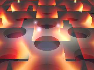
.... here is the render with patterning showing the overlap problem ...
Post a reply to this message
Attachments:
Download 'phc_and_excitation_enhancement.png' (254 KB)
Preview of image 'phc_and_excitation_enhancement.png'
|
|
| |
| |
|
|
|
|
| |
| |
|
|
.... and here is a zip with the scene again and the df3 files.
Post a reply to this message
Attachments:
Download 'pov_scene_and_df3s.zip' (212 KB)
|
|
| |
| |
|
|
|
|
| |
| |
|
|
"cbpypov" <nomail@nomail> wrote:
> I further set the QD absorption to 0. as Bald Eagle suggested. I really like the
> arrow thing you posted, but somehow I could not figure out where the `Vector`
> function comes from? My povray does not know it and I could not find an .inc
> that defines it. Could you post more code that you used for the image with
> arrows?
That's from Friedrich Lohmueller's analytical_g.inc file, which I _think_ comes
with POV-Ray.
http://www.f-lohmueller.de/pov_tut/addon/00_Basic_Templates/85_Analytical_Geo/__index.htm
> In the next to posts I will attach an image of the _patterned_ version, which is
> not working yet because the boxes in which the field is defined overlap. How can
> I solve this problem?
difference {} away the parts that overlap?
Post a reply to this message
|
|
| |
| |
|
|
|
|
| |
| |
|
|
I had that as part of a mental list to post, but it slipped off...
I was also thinking that if you wanted to represent an emission, you ought to
use the standard lambda-photon-sine-wave thing
like
https://physics.aps.org/assets/5f985b1a-28d8-4cb1-89f1-1ae7dedeac6f/e135_2_thumb.png
Just define it as an object that you can replace that quickie Vector () with.
And now I'm off to lunch.
Post a reply to this message
|
|
| |
| |
|
|
|
|
| |
|
|