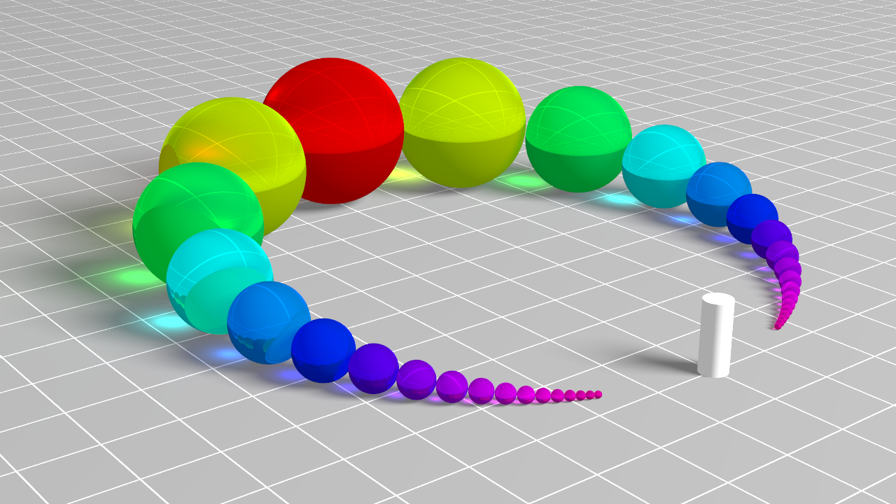
|
|
|
|
|
|
| |
| |
|
|
|
|
| |
| |
|
|
I threw together this little inversive geometry doodle last night to just make
something fun after a long while.

I might do some Steiner porisms and Appolonian gasket type stuff at some point.
Hoping some hyperbolic geometry on a Poisson disk.

I think a plane-filling Appolonian gasket pattern would be super cool, with an
inversion iteration level as a pattern argument.

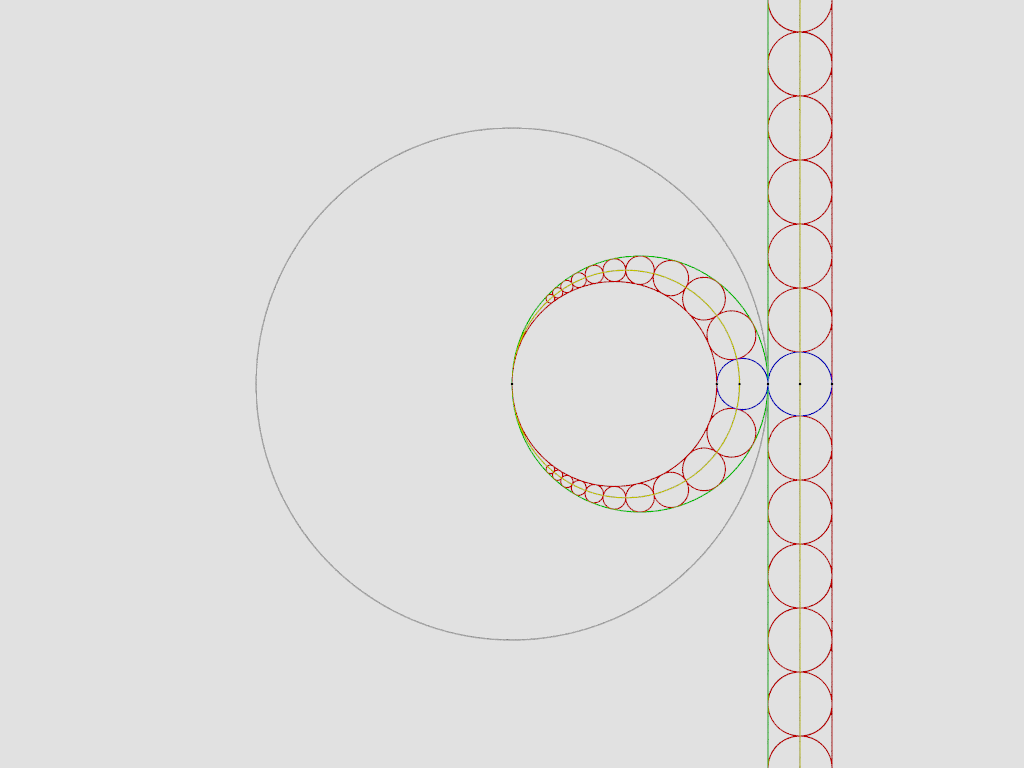
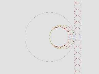
Anyway, what's going on here is that things that are defined IN the gray circle,
get inverted to the outside of the circle.  Circles not passing through the
center of the inversion circle stay circles, and circles passing through the
center get inverted to lines (circles of infinite radius).  Tangency is
preserved.

Likewise, objects defined outside of the circle get inverted to the inside of
the gray circle.

The closer things are to the circle, the closer they are inverted, and the
closer they are to the center, the farther away they are, and the center maps to
"a point at infinity".

Rather than doing several pages of Euclidean geometry like Pappus, we use Felix
Klein's inversive geometry to leverage the special properties mentioned above.

We make 2 circles that pass through the center, and so get mapped to lines.
A circle tangent to both of those circles (blue) gets mapped to a circle outside
the inversion circle, and is tangent to the 2 lines from the inverted circles.
Then, since all of the subsequent circles are tangent to both of the circles and
the small circle next to it, they are easily made as circles outside the
inversion circle that are all just stacked circles of the same radius - they are
tangent to both lines and the circles next to them.
So when they get inverted to the inside of the circle, they preserve those
properties of tangency.

And out pops a Pappus chain.  Easy peasy.

- BE
Post a reply to this message
Attachments:
Download 'pappuschain.png' (75 KB)
Preview of image 'pappuschain.png'
|
|
| |
| |
|
|
|
|
| |
| |
|
|
On 5/28/24 19:41, Bald Eagle wrote:
> And out pops a Pappus chain.
Cool!

Bill P.
Post a reply to this message
|
|
| |
| |
|
|
|
|
| |
| |
|
|
William F Pokorny <ano### [at] anonymous org> wrote:
> Cool!
Isn't it?
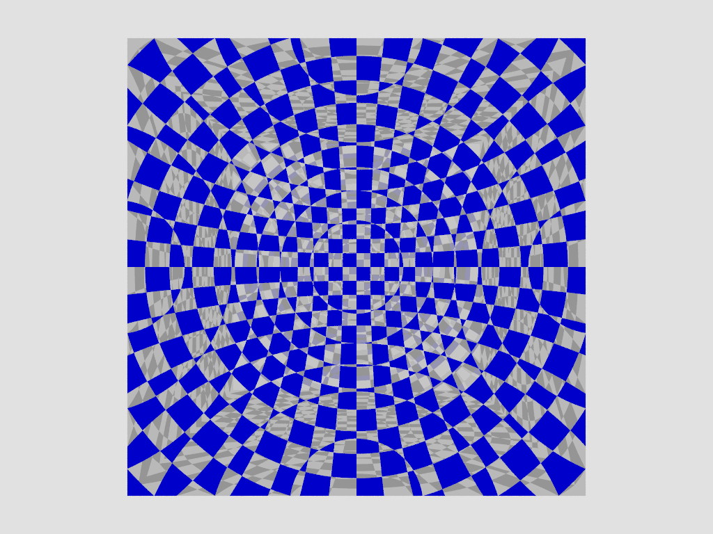
You can invert anything, even whole patterns, like so:
#declare Inversion = function {Radius*Radius / ( pow (x-CenterX, 2) + pow
(y-CenterY, 2) + pow (z-CenterZ, 2))}
#declare Checker_Inv = function {
Checker (
x*Inversion (x, y, z),
y*Inversion (x, y, z),
z*Inversion (x, y, z)
).red
}
plane {z, 0 pigment {function {Checker_Inv (x, y, z)}}}
I was trying to figure out a way to plug this into a matrix transform, but
POV-Ray doesn't allow that kind of thing.
/*
#declare M_Inversion =
function {
transform {
matrix <
Inversion (x, y, z), 0, 0,
0, Inversion (x, y, z), 0,
0, 0, Inversion (x, y, z),
0, 0, 0
>
}
}
*/ org> wrote:
> Cool!
Isn't it?
You can invert anything, even whole patterns, like so:
#declare Inversion = function {Radius*Radius / ( pow (x-CenterX, 2) + pow
(y-CenterY, 2) + pow (z-CenterZ, 2))}
#declare Checker_Inv = function {
Checker (
x*Inversion (x, y, z),
y*Inversion (x, y, z),
z*Inversion (x, y, z)
).red
}
plane {z, 0 pigment {function {Checker_Inv (x, y, z)}}}
I was trying to figure out a way to plug this into a matrix transform, but
POV-Ray doesn't allow that kind of thing.
/*
#declare M_Inversion =
function {
transform {
matrix <
Inversion (x, y, z), 0, 0,
0, Inversion (x, y, z), 0,
0, 0, Inversion (x, y, z),
0, 0, 0
>
}
}
*/
Post a reply to this message
|
|
| |
| |
|
|
|
|
| |
| |
|
|
On 5/29/24 06:54, Bald Eagle wrote:
> You can invert anything, even whole patterns, like so:

Thanks for posting more detailed code. I played a little - and it's cool
- though the results kinda twist my head around at times. :-)

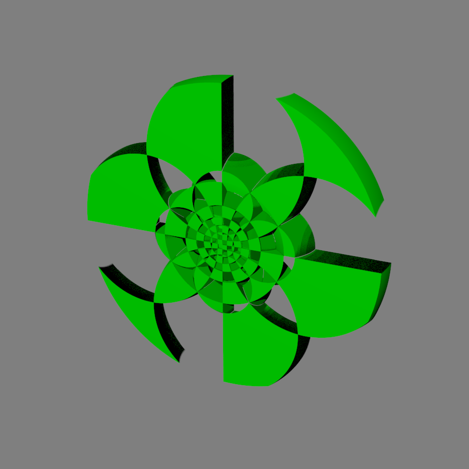
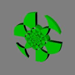
Attached is a slice of a sphere to the -z side of the x,y plane where
the radius of a f_sphere() is getting 'inverted / chopped' with your
'Checker_Inv()' (I also clamped the maximum Inversion() value to 15).
The sides sliced at the inversions don't render cleanly with the
isosurface, but we still end up with an interesting looking shape.

A little surprised it worked as well as it did...

Bill P.

FYI. I did get a few divisions by zero from Inversion() until I added
some off grid, anti-directional, numerical fuzz to CenterX, CenterY and
CenterZ. This might be due how my yuqk AA works compared to the
officially released AA.
Post a reply to this message
Attachments:
Download 'tmp2.png' (105 KB)
Preview of image 'tmp2.png'
|
|
| |
| |
|
|
|
|
| |
| |
|
|
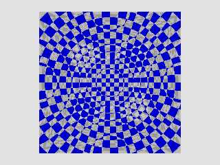
So that's very cool, and I wondered what it would look like if rendered as a
whole sphere, maybe with a glass texture and some sort of variation of the color
- perhaps determined by the Manhattan distance from the center.

I just used a quick, textured box, and the larger the inversion circle, the
smaller / more compact the pattern.   Patterns jump out at different scales.
Post a reply to this message
Attachments:
Download 'invertedpatternsphere.png' (262 KB)
Preview of image 'invertedpatternsphere.png'
|
|
| |
| |
|
|
|
|
| |
| |
|
|
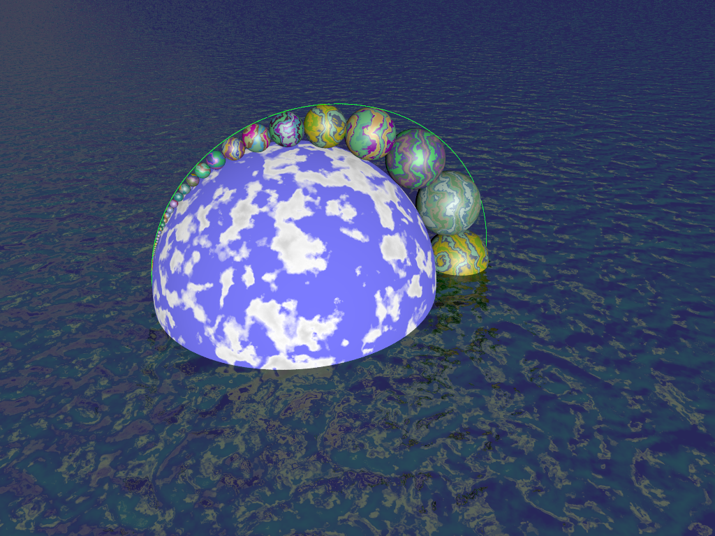
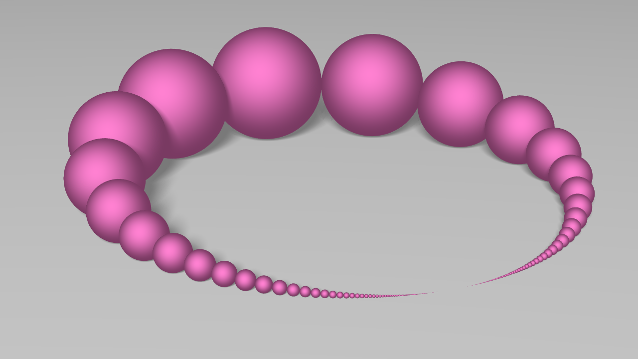
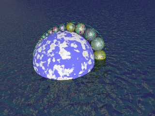
Ever inspired by the talented Francesco De Comite, I made a 3D version as a
little doodle.
Post a reply to this message
Attachments:
Download '3dpappuschain.png' (935 KB)
Preview of image '3dpappuschain.png'
|
|
| |
| |
|
|
|
|
| |
| |
|
|
On 12/06/2024 03:03, Bald Eagle wrote:
> Ever inspired by the talented Francesco De Comite, I made a 3D version as a
> little doodle.
>

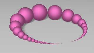
You have contaminated me ;)


--
Kurtz le pirate
Compagnie de la Banquise
Post a reply to this message
Attachments:
Download 'papus3.png' (201 KB)
Preview of image 'papus3.png'
|
|
| |
| |
|
|
|
|
| |
| |
|
|
kurtz le pirate <kur### [at] gmailcom> wrote:
> On 12/06/2024 03:03, Bald Eagle wrote:
> > Ever inspired by the talented Francesco De Comite, I made a 3D version as a
> > little doodle.
> >
>
> You have contaminated me ;)

You spelled "inspired" wrong.   :P

That's a beauty.
I'll bet that would amazing done in glass with caustics.
Or as stone spheres in a field of grass.

I still need to work out some good code for an Appolonian gasket.
(Unless you beat me to it  ;)  )

- BW
Post a reply to this message
|
|
| |
| |
|
|
|
|
| |
| |
|
|
"Bald Eagle" <cre### [at] netscapenet> wrote:

> I'll bet that would amazing done in glass with caustics.

Check out:

https://www.dumas.io/limset3d/
Post a reply to this message
|
|
| |
| |
|
|
|
|
| |
| |
|
|
On 12/06/2024 17:52, Bald Eagle wrote:
> I still need to work out some good code for an Appolonian gasket.
> (Unless you beat me to it  ;)  )


I'm working on it too.

wip here : <http://louisbel.free.fr/scenes/scene038.shtml>
(in french for the moment)


--
Kurtz le pirate
Compagnie de la Banquise
Post a reply to this message
|
|
| |
| |
|
|
|
|
| |
| |
|
|
On 12/06/2024 17:52, Bald Eagle wrote:

> That's a beauty.
Thanks

> I'll bet that would amazing done in glass with caustics.

Hum.. hum... lot of work.
I have to think about it

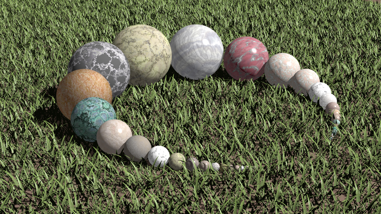
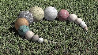
> Or as stone spheres in a field of grass.

Easier and faster. First test attached.
Does it match your idea ?


Note :
- Random textures from "stones.inc" without optimization
- Makegrass macro from Gilles Tran


--
Kurtz le pirate
Compagnie de la Banquise
Post a reply to this message
Attachments:
Download 'papus_grass.jpg' (1510 KB)
Preview of image 'papus_grass.jpg'
|
|
| |
| |
|
|
|
|
| |
| |
|
|
hi,

kurtz le pirate <kur### [at] gmailcom> wrote:
> ...
> wip here : {...}

the "l'image en noir et blanc" does it for me, v nice.


regards, jr.
Post a reply to this message
|
|
| |
| |
|
|
|
|
| |
| |
|
|
kurtz le pirate <kur### [at] gmailcom> wrote:

> I'm working on it too.
>
> wip here : <http://louisbel.free.fr/scenes/scene038.shtml>
> (in french for the moment)

Very nice.  Excellent work as always!
I see you've been going over the same references as I have.

I just started watching Daniel Schiffman's video this morning - I was hoping to
start writing some code based on it after work.

I'm still amazed that "Beyond the Descartes Circle Theorem" was only published
in 2001!  :O

I recall in one of the sites that I stumbled across, there was a method for
calculating how many circles there were for any given level of recursion.
That might be a nice addition to the debug stream, as well as warning/sanity
check before a render is attempted to be started with too high a level of
recursion for the system it's being run on.

It would also be nice to have a few ways to generate the output, so that the
gasket could be further used in a more complex scene.

1. Someone might want the tori to overlap such that the centers of their minor
radii are coincident/tangent, OR they might want the outside surfaces of the
tori to be tangent.

2. The coloration of each level of recursion ought to be able to be specified by
something like an array.  That way different textures and normals, etc can be
applied.  Also, it could then be rendered and subsequently used as a
heightfield.

3. There might be a desire to texture the circles based on their radius, or from
the distance from the center of the outer circle.

I've also found PDF and djvu copies of "Indra's Pearls" on the web, and they
have some very interesting algorithms to render a wide variety of variations on
this theme.

The authors even mention that some madman might be able to do this in Excel -
which is what I'm currently working on, since it's the only tool I have
available during the day.  :D

- BW
Post a reply to this message
|
|
| |
| |
|
|
|
|
| |
| |
|
|
On 13/06/2024 17:17, kurtz le pirate wrote:
> I'm working on it too.
> wip here : <http://louisbel.free.fr/scenes/scene038.shtml>

Really nice !
Especially metal-like construction on black.
Also math surfaces in Scenes menu attracted my attention - I love them
also.
--
YB
Post a reply to this message
|
|
| |
| |
|
|
|
|
| |
| |
|
|
On 6/13/24 10:17, kurtz le pirate wrote:
> wip here :<http://louisbel.free.fr/scenes/scene038.shtml>

Cool!

Bill P.
Post a reply to this message
|
|
| |
| |
|
|
|
|
| |
| |
|
|
"Bald Eagle" <cre### [at] netscapenet> wrote:

> I just started watching Daniel Schiffman's video this morning - I was hoping to
> start writing some code based on it after work.

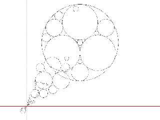
Well, I got partway there.
I'm botching _something_ up (as usual).

I need to stop blindly hacking and do some more thinking and learning.


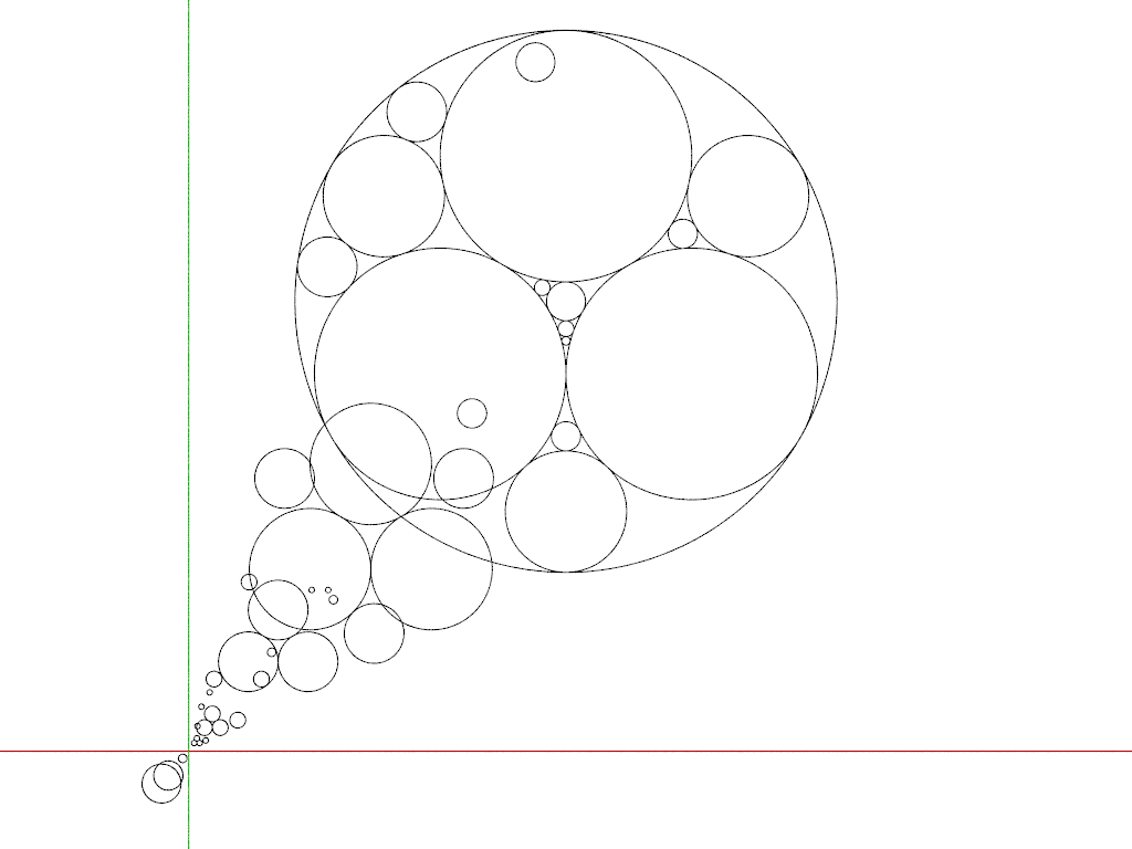
#version 3.8;
global_settings {assumed_gamma 1.0 }

#declare S3 = sqrt(3);

#declare M = 3;
#declare C1 = < 1,  0,  1>+M*(x+y);
#declare C2 = <-1,  0,  1>+M*(x+y);
#declare C3 = < 0, S3,  1>+M*(x+y);


camera {
 location M*<1, S3/2, -2.25>
 right x*image_width/image_height
 up y
 look_at M*<1, S3/2, 0>
 //rotate y*15
}
sky_sphere {pigment {rgb 1}}
light_source {< 0, 0, -150> rgb 1}

#declare Line = 0.005;

cylinder {-x*100, x*100, Line pigment {rgb x}}
cylinder {-y*100, y*100, Line pigment {rgb y}}

#declare k4curvature1 = function (k1, k2, k3) {k1 + k2 + k3 + 2 * sqrt (k1*k2 +
k2*k3 + k3*k1)}
#declare k4curvature2 = function (k1, k2, k3) {k1 + k2 + k3 - 2 * sqrt (k1*k2 +
k2*k3 + k3*k1)}


// Make every circle a vector: <Real, Imaginary, Radius>
// Start out with <R, I, 0> to do math, and then tack on radius in last step
// That way add, subtract, and scalar multiplication are all just operations on
a vector

#macro Re(Z) Z.x #end
#macro Im(Z) Z.y #end
#macro Mult(z1, z2) <Re(z1)*Re(z2) - Im(z1)*Im(z2), Re(z1)*Im(z2) +
Im(z1)*Re(z2)> #end

#macro Sqrt (Z)
 #local m = sqrt ( Re(Z)*Re(Z) + Im(Z)*Im(Z) );
 #local Angle = atan2 (Im(Z), Re(Z)) / 2;
 #local NewZ = sqrt(m)*<cos(Angle), sin(Angle)>;
 NewZ
#end

#macro ComplexDescartes (C1, C2, C3, k4)
 // z41 = (z1*k1 + z2*k2 + z3*k3 + 2 * sqrt (z1*k1*z2*k2 + z2*k2*z3*k3 +
z3*k3*z1*k1)) / k4
 // z42 = (z1*k1 + z2*k2 + z3*k3 - 2 * sqrt (z1*k1*z2*k2 + z2*k2*z3*k3 +
z3*k3*z1*k1)) / k4
 #local k1 = 1/C1.z;
 #local k2 = 1/C2.z;
 #local k3 = 1/C3.z;

 #local z1 = <C1.x, C1.y>;
 #local z2 = <C2.x, C2.y>;
 #local z3 = <C3.x, C3.y>;

 #local zk1 = z1*k1;
 #local zk2 = z2*k2;
 #local zk3 = z3*k3;

 #local Sum = zk1 + zk2 + zk3;
 #local Square = Mult (zk1, zk2) + Mult (zk2, zk3) + Mult (zk3, zk1);
 #local Root = Sqrt (Square);

 #local z41 = (Sum + 2*Root) / k4;
 #local z42 = (Sum - 2*Root) / k4;

 #local Z41 = z41 + <0, 0, 1/k4>;
 #local Z42 = z42 + <0, 0, 1/k4>;

 #local Result = array [2] {Z41, Z42};

 Result
#end

#macro Circle (C)
 torus {abs(C.z), Line pigment {rgb 0} rotate x*90 translate <C.x, C.y, 0>}
#end


#declare k41 = k4curvature1 (1/C1.z, 1/C2.z, 1/C3.z);
#declare k42 = k4curvature2 (1/C1.z, 1/C2.z, 1/C3.z);

#declare C41 = ComplexDescartes (C1, C2, C3, k41);
#declare C42 = ComplexDescartes (C1, C2, C3, k42);

#if (0)
Circle (C1)
Circle (C2)
Circle (C3)
Circle (C41[0])
Circle (C42[1])
#end

#macro DrawCircles (Array)
 #local Circles = dimension_size (Array, 1)-1;
 #for (C, 0, Circles)
  Circle (Array [C])
 #end
#end

#declare AllCircles = array;
#declare AllCircles [0] = C1;
#declare AllCircles [1] = C2;
#declare AllCircles [2] = C3;

#declare Queue = array;
#declare Queue [0] = array [3] {C1, C2, C3};

//#declare Queue [0] = C1;
//#declare Queue [1] = C2;
//#declare Queue [2] = C3;

#declare Levels = 3;

#macro Gasket (RecursionLevels)
 #for (L, 0, RecursionLevels)
  #local Triplets = dimension_size (Queue, 1)-1;
  #for (T, 0, Triplets)
   DrawCircles (Queue [T])
  #end

  #declare NextQueue = array;
  #local QIndex = 0;
  #for (T, 0, Triplets)
   #local triplet = Queue [T];
   #local c1 = triplet [0];
   #local c2 = triplet [1];
   #local c3 = triplet [2];
   #local k41 = k4curvature1 (1/c1.z, 1/c2.z, 1/c3.z);
   #local k42 = k4curvature2 (1/c1.z, 1/c2.z, 1/c3.z);
   #declare new1 = ComplexDescartes (c1, c2, c3, k41);
   #declare new2 = ComplexDescartes (c1, c2, c3, k42);

   #local T1 = array [3] {c1, c2, new1[0]};
   #local T2 = array [3] {c2, c3, new1[1]};
   #local T3 = array [3] {c3, c1, new1[1]};
   #local T4 = array [3] {c1, c2, new2[1]};
   #local T5 = array [3] {c2, c3, new2[1]};
   #local T6 = array [3] {c3, c1, new2[1]};
   //#local T6 = array [3] {c2, c3, new1[1]};

   #declare NextQueue [QIndex] = T1;
   #local QIndex = QIndex + 1;
   #declare NextQueue [QIndex] = T2;
   #local QIndex = QIndex + 1;
   #declare NextQueue [QIndex] = T3;

   #local QIndex = QIndex + 1;
   #declare NextQueue [QIndex] = T4;
   #local QIndex = QIndex + 1;
   #declare NextQueue [QIndex] = T5;
   #local QIndex = QIndex + 1;
   #declare NextQueue [QIndex] = T6;

  #end // end for T

  #declare Queue = NextQueue;
 #end // end for L
#end

Gasket (Levels)
Post a reply to this message
Attachments:
Download 'appolonian_gasket.png' (62 KB)
Preview of image 'appolonian_gasket.png'
|
|
| |
| |
|
|
|
|
| |
| |
|
|
"Bald Eagle" <cre### [at] netscapenet> wrote:

> Well, I got partway there.
> I'm botching _something_ up (as usual).

I almost got it.
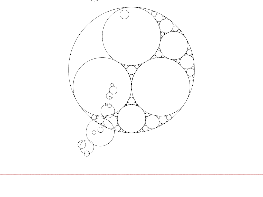
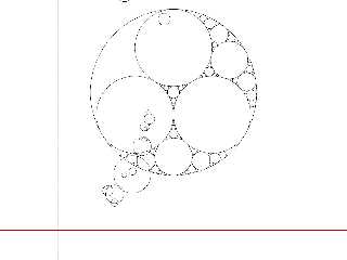
Removing one of the circle solutions cleaned up a bunch of unnecessary circles,
but the circles for the top right area are in the wrong place.
I'm wondering if there's some sign or floating point thing going on.

This is 5 levels of recursion.

Minor changes to recursion macro:
(mostly just 2 changes to an array index, restoring them to my initial values)

#macro Gasket (RecursionLevels)
 #for (L, 0, RecursionLevels)
  #local Triplets = dimension_size (Queue, 1)-1;
  #for (T, 0, Triplets)
   DrawCircles (Queue [T])
  #end

  #declare NextQueue = array;
  #local QIndex = 0;
  #for (T, 0, Triplets)
   #local triplet = Queue [T];
   #local c1 = triplet [0];
   #local c2 = triplet [1];
   #local c3 = triplet [2];
   #local k41 = k4curvature1 (1/c1.z, 1/c2.z, 1/c3.z);
   #local k42 = k4curvature2 (1/c1.z, 1/c2.z, 1/c3.z);
   #declare new1 = ComplexDescartes (c1, c2, c3, k41);
   #declare new2 = ComplexDescartes (c1, c2, c3, k42);

   #local T1 = array [3] {c1, c2, new1[0]};
   #local T2 = array [3] {c2, c3, new1[0]};//
   #local T3 = array [3] {c3, c1, new1[0]};//
   #local T4 = array [3] {c1, c2, new2[1]};
   #local T5 = array [3] {c2, c3, new2[1]};
   #local T6 = array [3] {c3, c1, new2[1]};
   //#local T6 = array [3] {c2, c3, new1[1]};

   #declare NextQueue [QIndex] = T1;
   #local QIndex = QIndex + 1;
   #declare NextQueue [QIndex] = T2;
   #local QIndex = QIndex + 1;
   #declare NextQueue [QIndex] = T3;

   #local QIndex = QIndex + 1;
   #declare NextQueue [QIndex] = T4;
   //#local QIndex = QIndex + 1;
   //#declare NextQueue [QIndex] = T5;
   #local QIndex = QIndex + 1;
   #declare NextQueue [QIndex] = T6;

  #end // end for T

  #declare Queue = NextQueue;
 #end // end for L
#end
Post a reply to this message
Attachments:
Download 'appolonian_gasket.png' (58 KB)
Preview of image 'appolonian_gasket.png'
|
|
| |
| |
|
|
|
|
| |
| |
|
|
"Bald Eagle" <cre### [at] netscapenet> wrote:

> I recall in one of the sites that I stumbled across, there was a method for
> calculating how many circles there were for any given level of recursion.
> That might be a nice addition to the debug stream, as well as warning/sanity
> check before a render is attempted to be started with too high a level of
> recursion for the system it's being run on.

https://en.wikibooks.org/wiki/Fractals/Apollonian_fractals
Post a reply to this message
|
|
| |
| |
|
|
|
|
| |
| |
|
|
A few quick explanations for those interested.
(I'd probably do a page on my site... but I'm so far behind ;) )


I haven't used Bald Eagle's inversion method, which looks very
interesting and promising.


The reference being the WIKIPEDIA page
<https://en.wikipedia.org/wiki/Pappus_chain>


-- The two basic radii :
#declare BigRadius = SIZE; // AB/2
#declare SmallRadius = SIZE*3/4; // AC/2


-- For the first circle (CB):
#declare cx = SmallRadius*2 + BigRadius - SmallRadius;
#declare r = BigRadius - SmallRadius;
DrawCircle(cx, 0, r)


-- Next, a simple loop :
#declare r = SmallRadius/BigRadius;
#declare NthRadius = r;

#declare n = 1;
#while ( NthRadius > MIN_RADIUS )
  #declare divisor = n*n*(1-r)*(1-r)+r;
  #declare xx = 2*BigRadius*r*(1+r)/(2*divisor);
  #declare yy = 2*BigRadius*n*r*(1-r)/divisor;
  #declare NthRadius = 2*BigRadius*r*(1-r)/(2*divisor);

  DrawCircle(xx, +yy, NthRadius)
  DrawCircle(xx, -yy, NthRadius) // symmetrically

  #declare n = n + 1;
#end


The first tests were in 2D. So I made a macro that drew circles :
#macro DrawCircle(X,Y,R,C)
 torus { R, rLine pigment { color C } rotate 90*x translate <X,Y,0> }
#end


Transformed for 3d :
#macro DrawCircle(X,Y,R,C)
 sphere { <X,R,Y>, R pigment { color C } }
#end


A yes, I forgot! The end of the loop is controlled by the constancy
MIN_RADIUS. If the radius is "too" small, we stop.

#declare MIN_RADIUS = 0.50; for the stone spheres


--
Kurtz le pirate
Compagnie de la Banquise
Post a reply to this message
|
|
| |
| |
|
|
|
|
| |
| |
|
|
On 14/06/2024 16:30, Bald Eagle wrote:
> "Bald Eagle" <cre### [at] netscapenet> wrote:
> https://en.wikibooks.org/wiki/Fractals/Apollonian_fractals

This guy is working on similar things and making interactive toys:
https://observablehq.com/@esperanc/3d-apollonian-sphere-packings
--
YB
Post a reply to this message
|
|
| |
| |
|
|
|
|
| |
| |
|
|
On 14/06/2024 19:30, yesbird wrote:
> This guy is working on similar things and making interactive toys:
> https://observablehq.com/@esperanc/3d-apollonian-sphere-packings

Also this paper may be of interest:
https://arxiv.org/pdf/1609.03811
--
YB
Post a reply to this message
|
|
| |
| |
|
|
|
|
| |
| |
|
|
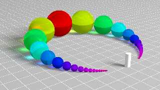
On 12/06/2024 17:52, Bald Eagle wrote:
> I'll bet that would amazing done in glass with caustics.
> Or as stone spheres in a field of grass.
>

After grass and stones, glass.


--
Kurtz le pirate
Compagnie de la Banquise
Post a reply to this message
Attachments:
Download 'papus4_colors_1.png' (349 KB)
Preview of image 'papus4_colors_1.png'
|
|
| |
| |
|
|
|
|
| |
| |
|
|
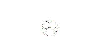
Ugh.

I tried rewriting from scratch (porting the Javascript code from
https://en.wikibooks.org/wiki/Fractals/Apollonian_fractals to SDL)
and I'm still stuck with that upper left hand portion not being right.

I thought maybe some of the quadratic solution checking in that could would fix
things, because saving that code as an SVG file and opening it in a browser
works beautifully (and it's FAST!).

So, still sitting here with my dunce cap on until I figure out how to wrap my
head around what's going wrong with the center coordinates and the recursion
queue.

- BW
Post a reply to this message
|
|
| |
| |
|
|
|
|
| |
| |
|
|
Am 16.06.2024 um 13:44 schrieb Bald Eagle:
> Ugh.
>
> I tried rewriting from scratch (porting the Javascript code from
> https://en.wikibooks.org/wiki/Fractals/Apollonian_fractals to SDL)
> and I'm still stuck with that upper left hand portion not being right.
>
> I thought maybe some of the quadratic solution checking in that could would fix
> things, because saving that code as an SVG file and opening it in a browser
> works beautifully (and it's FAST!).
>
> So, still sitting here with my dunce cap on until I figure out how to wrap my
> head around what's going wrong with the center coordinates and the recursion
> queue.
>
> - BW
>
It took me a while to understand this weird javascript recursion and I
mixed up some - with + or vice versa:

global_settings {assumed_gamma 1.0 }

#include "colors.inc"

#declare S3 = sqrt(3);

#declare M = 3;
#declare C1 = < 1,  0,  1>+M*(x+y);
#declare C2 = <-1,  0,  1>+M*(x+y);
#declare C3 = < 0, S3,  1>+M*(x+y);


camera {
  location M*<0,0,-2.25>//M*<1, S3/2, -2.25>
  right x*image_width/image_height
  up y
  look_at <0,0,0>//M*<1, S3/2, 0>
  //rotate y*15
}
sky_sphere {pigment {rgb 1}}
light_source {< 0, 0, -150> rgb 1}

#declare Line = 0.005;

cylinder {-x*100, x*100, Line pigment {rgb x}}
cylinder {-y*100, y*100, Line pigment {rgb y}}

#declare k4curvature1 = function (k1, k2, k3) {k1 + k2 + k3 + 2 * sqrt
(k1*k2 +
k2*k3 + k3*k1)}
#declare k4curvature2 = function (k1, k2, k3) {k1 + k2 + k3 - 2 * sqrt
(k1*k2 +
k2*k3 + k3*k1)}

#macro Re(Z) Z.x #end
#macro Im(Z) Z.y #end
#macro Cmul(z1, z2)
    <Re(z1)*Re(z2) - Im(z1)*Im(z2), Re(z1)*Im(z2) + Im(z1)*Re(z2)>
#end
#macro Cadd(a,b)
    <Re(a)+Re(b),Im(a)+Im(b)>
#end
#macro Csub(a,b)
    <Re(a)-Re(b),Im(a)-Im(b)>
#end

#macro Csqrt (Z)
  #local m = sqrt ( Re(Z)*Re(Z) + Im(Z)*Im(Z) );
  #local Angle = atan2 (Im(Z), Re(Z)) / 2;
  #local NewZ = sqrt(m)*<cos(Angle), sin(Angle)>;
  NewZ
#end
/*#macro Csqrt(Z)
    #local m = sqrt ( Re(Z)*Re(Z) + Im(Z)*Im(Z) );
    <sqrt((m+Re(Z))/2),abs(Im(Z))/Im(Z)*sqrt((m-Re(Z))/2)>
#end*/


#declare Colours=array[7]{Violet,Blue,Cyan,Green,Yellow,Orange,Red}

#macro DrawCircle (C,PigmNr)
    torus {abs(C.z), Line pigment {colour Colours[PigmNr]} rotate x*90
translate <C.x, C.y, 0>}
#end


/***********************************************
Edit the seed for other circles or run an animation
#declare Zufall=seed(36730+frame_number);
************************************************/

#declare Zufall=seed(36730+17);

// unit circle
#declare b=<0,0,-1>;

// insert two raqndomly positioned touching circles
#declare tr = 1-rand(Zufall)/2;
#declare pa = pi/2 - asin(rand(Zufall)*(1-tr)/tr);
#declare px = tr * cos(pa);
#declare py = tr * sin(pa);
#declare pr = 1 - tr;
#declare qr = (1 - pr) * (1 - cos(pa + pi/2))  / (1 + pr - (1 - pr)
*cos(pa + pi/2));
#declare qx = 0;
#declare qy = qr - 1;

#declare p=<px,py,pr>;
#declare q=<qx,qy,qr>;

#declare MinRadius=0.1;

#declare MaxDepth=7;

#macro Kiss(a,b,c,initial,Depth)
    #if (Depth <= MaxDepth)
       #local k1 = 1/a.z; // real
       #local z1 = <a.x,a.y>; // complex
       #local kz1 = Cmul(<k1,0>,z1); // complex

       #local k2 = 1/b.z; // real
       #local z2 = <b.x,b.y>; // complex
       #local kz2 = Cmul(<k2,0>,z2); // complex

       #local k3 = 1/c.z; // real
       #local z3 = <c.x,c.y>; // complex
       #local kz3 = Cmul(<k3,0>,z3); // complex

       #local k4p = k1 + k2 + k3 + 2*sqrt(k1*k2 + k2*k3 + k3*k1); // real
       #local k4m = k1 + k2 + k3 - 2*sqrt(k1*k2 + k2*k3 + k3*k1); // real

       #local kz4p =
Cadd(Cadd(Cadd(kz1,kz2),kz3),Cmul(<2,0>,Csqrt(Cadd(Cadd(Cmul(kz1,kz2),Cmul(kz2,kz3)),Cmul(kz3,kz1)))));

// complex
       #local kz4m =
Csub(Cadd(Cadd(kz1,kz2),kz3),Cmul(<2,0>,Csqrt(Cadd(Cadd(Cmul(kz1,kz2),Cmul(kz2,kz3)),Cmul(kz3,kz1)))));

// complex

       #if (k4p > k4m)
          #local k4 = k4p; // real
          #local kz4 = kz4p; // complex
          #local k4b = k4m; // real
          #local kz4b = kz4m; // complex
       #else
          #local k4 = k4m; // real
          #local kz4 = kz4m; // complex
          #local k4b = k4p; // real
          #local kz4b = kz4p; // complex
       #end

       #local cc = <kz4.x/k4 , kz4.y/k4 , abs(1/k4)>; // Circle

       #local dx = a.x - cc.x;
       #local dy = a.y - cc.y;
       #local dr = a.z + cc.z;

       #local dtest=abs(dx*dx + dy*dy - dr*dr);

       #if ( abs(dx*dx + dy*dy - dr*dr) > 0.0001 )
          #local cc = <kz4b.x/k4 , kz4b.y/k4 , abs(1/k4)>;
       #end

       #if (initial)
          #local cc=<kz4b.x/k4b,kz4b.y/k4b,abs(1/k4b)>;
       #end

       DrawCircle(cc,mod(Depth,7))

       Kiss(a,b,cc,false,Depth+1)
       Kiss(a,cc,c,false,Depth+1)
       Kiss(cc,b,c,false,Depth+1)
    #end
#end


DrawCircle(b,0)
DrawCircle(p,0)
DrawCircle(q,0)


Kiss(b,p,q,true,1)
Kiss(b,p,q,false,1)
Post a reply to this message
Attachments:
Download 'apollonian_fractals_03.png' (68 KB)
Preview of image 'apollonian_fractals_03.png'
|
|
| |
| |
|
|
|
|
| |
| |
|
|
MichaelJF <fri### [at] t-onlinede> wrote:

> It took me a while to understand this weird javascript recursion and I
> mixed up some - with + or vice versa:

Excellent!
Now that there's some working SDL, I can try to understand where things went off
the rails, and try to make some variations.

Maybe a nested Appolonian gasket, but also one with circles in between 2
straight lines (circles with infinite radius, curvature of zero, resulting in
"Ford circles)

Thanks so much, Michael!

- BW
Post a reply to this message
|
|
| |
| |
|
|
|
|
| |
| |
|
|
But for now...
Post a reply to this message
Attachments:
Download 'mjf_appolloniancylinders.png' (119 KB)
Preview of image 'mjf_appolloniancylinders.png'

|
|
| |
| |
|
|
|
|
| |
| |
|
|
And


#macro DrawCircle (C, PigmNr)

 //#debug concat( "C = ", vstr(3, C, ", ", 0, 3), " \n")
 //torus {abs(C.z), Line texture {pigment {colour Colours[PigmNr]} finish
{emission 1}} rotate x*90 translate <C.x, C.y, 0>}
 #if (C.z > 0 & C.z < 0.6)
 sphere {0, abs(C.z) scale <1, 1, 1+pow(abs(C.z), 0.001)> texture {pigment
{colour Colours[PigmNr]} finish {specular 0.4}} translate <C.x, C.y, 0>}
 #end
#end
Post a reply to this message
Attachments:
Download 'mjf_appollonianellipsoids.png' (133 KB)
Preview of image 'mjf_appollonianellipsoids.png'

|
|
| |
| |
|
|
|
|
| |
| |
|
|
And of course, because the Appollonian gasket is a foam, . . .

bubbles!
Post a reply to this message
Attachments:
Download 'mjf_appollonianbubbles.png' (608 KB)
Preview of image 'mjf_appollonianbubbles.png'

|
|
| |
| |
|
|
|
|
| |
| |
|
|
and with a nested gasket, we could do a sort of Sierpinski triangle.

There's some kind of transformation that makes them isomorphic.
Post a reply to this message
Attachments:
Download 'mjf_appolloniantriangles.png' (64 KB)
Preview of image 'mjf_appolloniantriangles.png'

|
|
| |
| |
|
|
|
|
| |
| |
|
|
On 17/06/2024 23:49, Bald Eagle wrote:
> Excellent!
> Now that there's some working SDL, I can try to understand where things went off
> the rails, and try to make some variations.


I've updated my page and published the code (at the very bottom).
<http://louisbel.free.fr/scenes/scene038.shtml>


Sorry, still in French
--
Kurtz le pirate
Compagnie de la Banquise
Post a reply to this message
|
|
| |
| |
|
|
|
|
| |
| |
|
|
On 18/06/2024 00:50, Bald Eagle wrote:
> And of course, because the Appollonian gasket is a foam, . . .
>
> bubbles!
>


GREAT Bubbles. Very good job.


--
Kurtz le pirate
Compagnie de la Banquise
Post a reply to this message
|
|
| |
| |
|
|
|
|
| |
| |
|
|
Just posting this here for reference.

https://www.johndcook.com/blog/2023/12/19/conformal-map-disk-triangle/

Would be cool to apply this to the gasket to see what pops out - probably a
Sierpinski Triangle.

Search: conformal mapping of circle to a triangle

- BE
Post a reply to this message
|
|
| |
| |
|
|
|
|
| |
| |
|
|
Now with lenses!
Post a reply to this message
Attachments:
Download 'mjf_appollonianlenses.png' (451 KB)
Preview of image 'mjf_appollonianlenses.png'

|
|
| |
| |
|
|
|
|
| |
| |
|
|
Am 19.06.2024 um 02:36 schrieb Bald Eagle:
> Now with lenses!
somewhat crazy, but very interesting;)

Best regards
Michael
Post a reply to this message
|
|
| |
| |
|
|
|
|
| |
| |
|
|
MichaelJF <fri### [at] t-onlinede> wrote:

> somewhat crazy, but very interesting;)

Aw, thanks Michael!

But what about the render?    :D
Post a reply to this message
|
|
| |
| |
|
|
|
|
| |
| |
|
|
On 6/19/24 09:17, Bald Eagle wrote:
> MichaelJF <fri### [at] t-onlinede> wrote:
>
>> somewhat crazy, but very interesting;)
>
> Aw, thanks Michael!
>
> But what about the render?    :D
>

You have too much free times... :-) Very cool.

Bill P.
Post a reply to this message
|
|
| |
| |
|
|
|
|
| |
| |
|
|
"Bald Eagle" <cre### [at] netscapenet> wrote:
> Just posting this here for reference.
>
> https://www.johndcook.com/blog/2023/12/19/conformal-map-disk-triangle/
>
> Would be cool to apply this to the gasket to see what pops out - probably a
> Sierpinski Triangle.
>
> Search: conformal mapping of circle to a triangle
>
> - BE

https://www.mathworks.com/matlabcentral/fileexchange/35008-generation-of-random-variates

https://www.mathworks.com/matlabcentral/fileexchange/1844-gaussian-hypergeometric-function

function z=hypergeometric2f1(a,b,c,x,n)
% HYPERGEOMETRIC2F1 Computes the hypergeometric function
% using a series expansion:
%
%    f(a,b;c;x)=
%
%    1 + [ab/1!c]x + [a(a+1)b(b+1)/2!c(c+1)]x^2 +
%    [a(a+1)(a+2)b(b+1)(b+2)/3!c(c+1)(c+2)]x^3 + ...
%
% The series is expanded to n terms
%
% This function solves the Gaussian Hypergeometric Differential Equation:
%
%     x(1-x)y'' + {c-(a+b+1)x}y' - aby = 0
%
% The Hypergeometric function converges only for:
% |x| < 1
% c != 0, -1, -2, -3, ...
%
%
% Comments to:
% Diego Garcia   - d.g### [at] ieeeorg
% Chuck Mongiovi - mon### [at] fastnet
% June 14, 2002
if nargin ~= 5
    error('Usage: hypergeometric2f1(a,b,c,x,n) --> Wrong number of arguments')
end
if (n <= 0 | n ~= floor(n))
    error('Usage: hypergeometric2f1(a,b,c,x,n) --> n has to be a positive
integer')
end
if (abs(x) > 1)
    error('Usage: hypergeometric2f1(a,b,c,x,n) --> |x| has to be less than 1')
end
if (c <= 0 & c == floor(c))
    error('Usage: hypergeometric2f1(a,b,c,x,n) --> c != 0, -1, -2, -3, ...')
end
z = 0;
m = 0;
while (m<n)
    if (m == 0)
        delta = 1;
    else
        delta = delta .* x .* (a + (m - 1)) .* (b + (m-1)) ./ m ./ (c + (m-1));
   end
   z = z + delta;
   m = m + 1;
end
Post a reply to this message
|
|
| |
| |
|
|
|
|
| |
| |
|
|
And of course we needed so good old fashioned crop circles.
(WIP)
Post a reply to this message
Attachments:
Download 'mjf_appolloniancropcircles.png' (828 KB)
Preview of image 'mjf_appolloniancropcircles.png'

|
|
| |
| |
|
|
|
|
| |
| |
|
|
Any python coders capable of converting this to SDL?

https://people.sc.fsu.edu/~jburkardt/py_src/hyper_2f1/hyper_2f1.py

#! /usr/bin/env python3
#
def hyper_2f1_test ( ):

#*****************************************************************************80
#
## hyper_2f1_test() tests hyper_2f1().
#
#  Licensing:
#
#    This code is distributed under the MIT license.
#
#  Modified:
#
#    21 December 2023
#
#  Author:
#
#    John Burkardt
#
  import platform

  print ( '' )
  print ( 'hyper_2f1_test():' )
  print ( '  Python version: %s' % ( platform.python_version ( ) ) )
  print ( '  Test hyper_2f1().' )

  hyper_2f1_real_test ( )
  hyper_2f1_complex_test ( )
#
#  Terminate.
#
  print ( '' )
  print ( 'hyper_2f1_test():' )
  print ( '  Normal end of execution.' )
  return

def hyper_2f1 ( a, b, c, x ):

#*****************************************************************************80
#
## hyper_2f1() evaluates the hypergeometric 2F1 function.
#
#  Licensing:
#
#    This code is distributed under the MIT license.
#
#  Modified:
#
#    21 December 2023
#
#  Author:
#
#    John Burkardt
#
#  Input:
#
#    real A, B, C: the parameters.
#
#    real or complex X: the argument.
#
#  Output:
#
#    real or complex F: the value of the function.
#
  from scipy.special import hyp2f1

  f = hyp2f1 ( a, b, c, x )

  return f

def hyper_2f1_real_values ( n_data ):

#*****************************************************************************80
#
## hyper_2f1_real_values() returns some values of the hypergeometric 2F1
function.
#
#  Discussion:
#
#    In Mathematica, the function can be evaluated by:
#
#      fx = Hypergeometric2F1 [ a, b, c, x ]
#
#  Licensing:
#
#    This code is distributed under the MIT license.
#
#  Modified:
#
#    13 February 2015
#
#  Author:
#
#    John Burkardt
#
#  Reference:
#
#    Milton Abramowitz, Irene Stegun,
#    Handbook of Mathematical Functions,
#    National Bureau of Standards, 1964,
#    ISBN: 0-486-61272-4,
#    LC: QA47.A34.
#
#    Shanjie Zhang, Jianming Jin,
#    Computation of Special Functions,
#    Wiley, 1996,
#    ISBN: 0-471-11963-6,
#    LC: QA351.C45
#
#    Stephen Wolfram,
#    The Mathematica Book,
#    Fourth Edition,
#    Cambridge University Press, 1999,
#    ISBN: 0-521-64314-7,
#    LC: QA76.95.W65.
#
#    Daniel Zwillinger, editor,
#    CRC Standard Mathematical Tables and Formulae,
#    30th Edition,
#    CRC Press, 1996,
#    ISBN: 0-8493-2479-3,
#    LC: QA47.M315.
#
#  Input:
#
#    integer n_data.  The user sets n_data to 0 before the first call.
#
#  Output:
#
#    integer n_data.  On each call, the routine increments n_data by 1, and
#    returns the corresponding data; when there is no more data, the
#    output value of n_data will be 0 again.
#
#    real A, B, C, X, the parameters.
#
#    real F, the value of the function.
#
  import numpy as np

  n_max = 24

  a_vec = np.array ( ( \
   -2.5, \
   -0.5, \
    0.5, \
    2.5, \
   -2.5, \
   -0.5, \
    0.5, \
    2.5, \
   -2.5, \
   -0.5, \
    0.5, \
    2.5, \
    3.3, \
    1.1, \
    1.1, \
    3.3, \
    3.3, \
    1.1, \
    1.1, \
    3.3, \
    3.3, \
    1.1, \
    1.1, \
    3.3 ))

  b_vec = np.array ( ( \
    3.3, \
    1.1, \
    1.1, \
    3.3, \
    3.3, \
    1.1, \
    1.1, \
    3.3, \
    3.3, \
    1.1, \
    1.1, \
    3.3, \
    6.7, \
    6.7, \
    6.7, \
    6.7, \
    6.7, \
    6.7, \
    6.7, \
    6.7, \
    6.7, \
    6.7, \
    6.7, \
    6.7 ))

  c_vec = np.array ( ( \
    6.7, \
    6.7, \
    6.7, \
    6.7, \
    6.7, \
    6.7, \
    6.7, \
    6.7, \
    6.7, \
    6.7, \
    6.7, \
    6.7, \
   -5.5, \
   -0.5, \
    0.5, \
    4.5, \
   -5.5, \
   -0.5, \
    0.5, \
    4.5, \
   -5.5, \
   -0.5, \
    0.5, \
    4.5 ))

  f_vec = np.array ( ( \
    0.72356129348997784913, \
    0.97911109345277961340, \
    1.0216578140088564160, \
    1.4051563200112126405, \
    0.46961431639821611095, \
    0.95296194977446325454, \
    1.0512814213947987916, \
    2.3999062904777858999, \
    0.29106095928414718320, \
    0.92536967910373175753, \
    1.0865504094806997287, \
    5.7381565526189046578, \
    15090.669748704606754, \
   -104.31170067364349677, \
    21.175050707768812938, \
    4.1946915819031922850, \
    1.0170777974048815592E+10, \
   -24708.635322489155868, \
    1372.2304548384989560, \
    58.092728706394652211, \
    5.8682087615124176162E+18, \
   -4.4635010147295996680E+08, \
    5.3835057561295731310E+06, \
    20396.913776019659426 ))

  x_vec = np.array ( ( \
    0.25, \
    0.25, \
    0.25, \
    0.25, \
    0.55, \
    0.55, \
    0.55, \
    0.55, \
    0.85, \
    0.85, \
    0.85, \
    0.85, \
    0.25, \
    0.25, \
    0.25, \
    0.25, \
    0.55, \
    0.55, \
    0.55, \
    0.55, \
    0.85, \
    0.85, \
    0.85, \
    0.85 ))

  if ( n_data < 0 ):
    n_data = 0

  if ( n_max <= n_data ):
    n_data = 0
    a = 0
    b = 0
    c = 0.0
    x = 0.0
    f = 0.0
  else:
    a = a_vec[n_data]
    b = b_vec[n_data]
    c = c_vec[n_data]
    x = x_vec[n_data]
    f = f_vec[n_data]
    n_data = n_data + 1

  return n_data, a, b, c, x, f

def hyper_2f1_real_test ( ):

#*****************************************************************************80
#
## hyper_2f1_real_test() tests hyper_2f1() for real arguments.
#
#  Licensing:
#
#    This code is distributed under the MIT license.
#
#  Modified:
#
#    21 December 2023
#
#  Author:
#
#    John Burkardt
#
  print ( '' )
  print ( 'hyper_2f1_real_test():' )
  print ( '  hyper_2f1() evaluates the hypergeometric function 2F1(A,B,C;X)' )
  print ( '  Check the computation for real arguments X.' )

  n_data = 0

  while ( True ):

    n_data, a, b, c, x, f1 = hyper_2f1_real_values ( n_data )

    if ( n_data == 0 ):
      break

    f2 = hyper_2f1 ( a, b, c, x )

    print ( '' )
    print ( '  (a,b,c,x):   %4d  %4d  %12f  %12f' % ( a, b, c, x ) )
    print ( '  (exact):     %24.16g' % ( f1 ) )
    print ( '  (computed):  %24.16g' % ( f2 ) )
    print ( '  (error):     %24.16g' % ( abs ( f1 - f2 ) ) )

  return

def hyper_2f1_complex_values ( n_data ):

#*****************************************************************************80
#
## hyper_2f1_complex_values() returns some values of the hypergeometric 2F1
function.
#
#  Discussion:
#
#    In Mathematica, the function can be evaluated by:
#
#      fz = Hypergeometric2F1 [ a, b, c, z ]
#
#  Licensing:
#
#    This code is distributed under the MIT license.
#
#  Modified:
#
#    19 December 2023
#
#  Author:
#
#    John Burkardt
#
#  Reference:
#
#    Shanjie Zhang, Jianming Jin,
#    Computation of Special Functions,
#    Wiley, 1996,
#    ISBN: 0-471-11963-6,
#    LC: QA351.C45
#
#  Input:
#
#    integer n_data.  The user sets n_data to 0 before the first call.
#
#  Output:
#
#    integer n_data.  On each call, the routine increments n_data by 1, and
#    returns the corresponding data; when there is no more data, the
#    output value of n_data will be 0 again.
#
#    real A, B, C: the parameters.
#
#    complex Z: the argument.
#
#    complex FZ: the value of the function.
#
  import numpy as np

  n_max = 15

  a_vec = np.array ( ( \
    3.2, \
    3.2, \
   -5.0, \
    3.3, \
   -7.0, \
    4.3, \
    3.3, \
    3.5, \
    3.3, \
    7.0, \
    5.0, \
    3.5, \
    2.1, \
    8.7, \
    8.7 ))

  b_vec = np.array ( ( \
   1.8, \
  -1.8, \
   3.3, \
  -6.0, \
   3.3, \
  -8.0, \
   5.8, \
  -2.4, \
   4.3, \
   5.0, \
   7.0, \
   1.2, \
   5.4, \
   3.2, \
   2.7 ))

  c_vec = np.array ( ( \
   6.7, \
   6.7, \
   6.7, \
   3.7, \
  -3.7, \
  -3.7, \
   6.7, \
   6.7, \
   6.7, \
   4.1, \
   4.1, \
   9.7, \
   9.7, \
   6.7, \
   6.7 ))

  fz_vec = np.array ( ( \
    5.468999154361234+0.00000000j, \
    0.3375063477462785+0.00000000j, \
    116.8274991533609+603.8909562709345j, \
    17620.41819334182+38293.80901310932j, \
   -11772775115.27448-14382285977.20268j, \
    1316118577866.058-101298889382.4362j, \
    1.733055678355656+0.6340102904953357j, \
    0.6476224071999852-0.5211050690999773j, \
   -1.483008322270093+8.374426179451589j, \
   -0.004037609523971226-0.002956632645480181j, \
   -0.004037609523971226-0.002956632645480181j, \
    1.034313610729953+0.5447389238499308j, \
    0.6885043978280027+1.227418679098749j, \
   -0.9004649679297319-1.11988994714304j, \
   -0.4608388640599718-0.5457569650549665j ))

  z_vec = np.array ( ( \
   1.0+0.0j, \
   1.0+0.0j, \
   5.2+4.8j, \
   5.2-4.8j, \
   5.2-4.8j, \
   5.2+4.8j, \
   0.2+0.1j, \
   0.2+0.5j, \
   0.8+0.3j, \
   3.0-1.0j, \
   3.0-1.0j, \
   0.6+0.9j, \
   0.5+0.7j, \
   0.5+0.7j, \
   0.6+0.9j ))

  if ( n_data < 0 ):
    n_data = 0

  if ( n_max <= n_data ):
    n_data = 0
    a = 0
    b = 0
    c = 0.0
    z = 0.0
    fz = 0.0
  else:
    a = a_vec[n_data]
    b = b_vec[n_data]
    c = c_vec[n_data]
    z = z_vec[n_data]
    fz = fz_vec[n_data]
    n_data = n_data + 1

  return n_data, a, b, c, z, fz

def hyper_2f1_complex_test ( ):

#*****************************************************************************80
#
## hyper_2f1_complex_test() tests hyper_2f1() for complex arguments.
#
#  Licensing:
#
#    This code is distributed under the MIT license.
#
#  Modified:
#
#    21 December 2023
#
#  Author:
#
#    John Burkardt
#
  print ( '' )
  print ( 'hyper_2f1_complex_test():' )
  print ( '  Test hyper_2f1() for complex arguments.' )

  n_data = 0

  while ( True ):

    n_data, a, b, c, z, f1 = hyper_2f1_complex_values ( n_data )

    if ( n_data == 0 ):
      break

    f2 = hyper_2f1 ( a, b, c, z )

    print ( '' )
    print ( '  (a,b,c,z):   %4d  %4d  %8f  (%8f,%8f)' % ( a, b, c, z.real,
z.imag ) )
    print ( '  (exact):     (%24.16g,%24.16g)' % ( f1.real, f1.imag ) )
    print ( '  (computed):  (%24.16g,%24.16g)' % ( f2.real, f2.imag ) )
    print ( '  (error):     %24.16g' % ( abs ( f1 - f2 ) ) )

  return

def timestamp ( ):

#*****************************************************************************80
#
## timestamp() prints the date as a timestamp.
#
#  Licensing:
#
#    This code is distributed under the MIT license.
#
#  Modified:
#
#    06 April 2013
#
#  Author:
#
#    John Burkardt
#
  import time

  t = time.time ( )
  print ( time.ctime ( t ) )

  return

if ( __name__ == '__main__' ):
  timestamp ( )
  hyper_2f1_test ( )
  timestamp ( )
Post a reply to this message
|
|
| |
| |
|
|
|
|
| |
| |
|
|
In my opinion, a special case was still missing here...

Blue is an osculatory sphere packing with an asymmetric start
configuration, red is a classical apollonian sphere packing with a
symmetric start configuration.

Best regards,
MIchael
Post a reply to this message
Attachments:
Download '20240724_apollonian_spheres_01b_1920.png' (528 KB)
Preview of image '20240724_apollonian_spheres_01b_1920.png'

|
|
| |
| |
|
|
|
|
| |
| |
|
|
On 24/07/2024 20:31, MichaelJF wrote:
> In my opinion, a special case was still missing here...
>
> Blue is an osculatory sphere packing with an asymmetric start
> configuration, red is a classical apollonian sphere packing with a
> symmetric start configuration.
>
> Best regards,
> MIchael
>

Waouh ! I'm always amazed by these kind of images.

Personally, I've never really understood the transition from plane work
to sphere work.


Excellent


--
Kurtz le pirate
Compagnie de la Banquise
Post a reply to this message
|
|
| |
| |
|
|
|
|
| |
| |
|
|
MichaelJF <fri### [at] t-onlinede> wrote:
> In my opinion, a special case was still missing here...
>
> Blue is an osculatory sphere packing with an asymmetric start
> configuration, red is a classical apollonian sphere packing with a
> symmetric start configuration.
>
> Best regards,
> MIchael


Yes, eventually we had to do the 3D version!
I had some papers on my pile (Well, _one_ of my piles) related to this.

How much more difficult was it to do the spherical space-filling version?


I'm also curious if this can be massaged into a macro that is capable of filling
any given arbitrary shape.

Then we could use it to build stone walls, layered geologic strata, sandstone
sculptures, etc.

Do a test scene with smooth spheres, and then enhance it by replacing them all
with isosurface rocks, pebbles, and sand.

A bowl of grapes.   That sort of thing.   :)


Excellent work - you ought to be proud.

- BW
Post a reply to this message
|
|
| |
| |
|
|
|
|
| |
| |
|
|
I plugged a prompt into the AI at work, just to see what sort of quality the
code and algorithms the thing spit out - and they're not all that terrible.

So I got some Ford Circles worked out (not using inversion).


Now, even this small experiment taught me some things.

spherical warp requires "orientation" and "dist_exp" to work properly,
especially as an interior_texture - otherwise you just get bad results.


And somehow, there may be a bug somewhere, or I'm just picking up some oddity in
the way the scene elements interact with each other - because I'm getting odd
"checkering" on that left-hand large sphere.   The crackle normal gets
flattened/canceled out.

If I remove the large, enclosing checkered sphere, it goes away.

Enjoy.

// ------------------------------------------------------------------------


#version 3.8;
global_settings {
 assumed_gamma 1.0
}
//#default {finish {emission 1}}
#declare E = 0.00001;

camera {
 location <0.5, 0.5, -1.75>
 right x*image_width/image_height
 up y
 look_at <0.5, 0.5, 0>
}

//sky_sphere {pigment {rgb 1}}
#declare BW = pigment_map
{
 [0 rgb 0]
 [1 rgb 1]
}

sphere {0, 1000 texture {pigment {checker rgb 0 rgb 1 scale x*0.5 warp
{spherical orientation y dist_exp 0.75} scale 1 }} } //interior_texture {pigment
{checker  scale 1 }} }

light_source {<5, 5, -50> rgb 1}

#declare Line = 0.001;

#declare Seed1 = seed (123);
#declare Seed2 = seed (456123);
#declare Seed3 = seed (456123789);

#macro FordCircle (p, q, mode)
 #local R1 = rand (Seed1);
 #local R2 = rand (Seed2);
 #local R3 = rand (Seed3);
 #local Color = <R1, R2, R3>;

 #local Radius = 1 / (2*pow(q,2));
 #local Center = <p/q, Radius, 0>;

 #switch (mode)
 #case (0)
  torus {Radius, Line pigment {rgb y} rotate x*90 translate Center}
  torus {Radius, Line pigment {rgb y} rotate x*90 translate <1, -1, 1>*Center
translate y*1}
 #break
 #case (1)
  disc {Center, z, Radius, 0 pigment {rgb Color}}
  disc {Center, z, Radius, 0 pigment {rgb Color} translate <0, 1-Radius*2, 0>}
 #break
 #case (2)
  sphere {Center, Radius texture {pigment {rgb Color} normal {crackle scale 0.01
bump_size 2} finish {specular 0.4}} }
  sphere {Center, Radius texture {pigment {rgb Color} normal {crackle scale
0.01} finish {specular 0.4}} translate <0, 1-Radius*2, 0>}
 #break
 #end
#end

#macro gcd (a, b)
 #if (b = 0)
  #local Result = a;
 #else
  #local Result = gcd (b, mod (a, b));
 #end
 Result
#end

#declare max_q = 10;

#for (q, 1, max_q)
 #for (p, 0, q)
  #if (gcd (p, q) = 1)
   FordCircle (p, q, 2)
  #end
 #end
#end
Post a reply to this message
Attachments:
Download 'fordcircles_ai.png' (824 KB)
Preview of image 'fordcircles_ai.png'

|
|
| |
| |
|
|
|
|
| |
| |
|
|
MichaelJF <fri### [at] t-onlinede> wrote:
> In my opinion, a special case was still missing here...
>
> Blue is an osculatory sphere packing with an asymmetric start
> configuration, red is a classical apollonian sphere packing with a
> symmetric start configuration.
>
> Best regards,
> MIchael

https://www.josleys.com/articles/Sphere_inversion_Article.pdf
Post a reply to this message
|
|
| |
| |
|
|
|
|
| |
|
|