 |
 |
|
 |
|
 |
|  |
|  |
|
 |
|
 |
|  |
|  |
|
 |
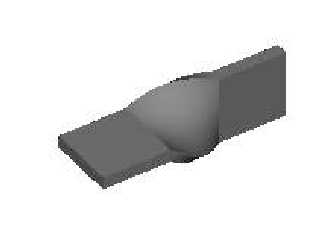
I would like to represent a length of metal 1 inch wide by 3/16 inch thick
that has a 90 degree twist over a 1 inch length.
Following the examples in the documentation (6.5.4.3.7 for twist) I have the
basic shape, but would prefer a less dramatic change from straight to twist.
Can the twist function be changed to start with no rotation, quickly
increase to the desired turns/unit and then back to no rotation?
Stephen
background { color <1.000,1.000,1.000> }
camera {
location < -58.033, -87.696, 83.175>
sky < 0.00000, 0.00000, 1.00000>
up < 0.0, 0.0, 1.0>
right < 1.33343, 0.0, 0.0>
angle 2.56896
look_at < -3.480, -4.962, 4.713>
}
light_source {
<0.0, 0.0, 0.0>
color rgb <1.000, 1.000, 1.000>
translate <-65.474138, -85.344511, 105.18157>
}
#local fn_A=function{abs(x)-.5};
#local fn_B=function{abs(z)-3/16/2};
#local fn_C=function{abs(y)-.5};
#local N=.25;
#local fn_twistY=function{z*sin(x*2*pi*N) + y*cos(x*2*pi*N)};
#local fn_twistZ=function{z*cos(x*2*pi*N) - y*sin(x*2*pi*N)};
#local fn_twist_Box=function{
max(
fn_A(x-.5,y,z),
fn_B(x,fn_twistY(x,y,z),fn_twistZ(x,y,z)),
fn_C(x,fn_twistY(x,y,z),fn_twistZ(x,y,z))
)
};
#local fn_Box=function{max(fn_A(x,y,z),fn_B(x,y,z),fn_C(x,y,z))};
isosurface {
function {
min(fn_Box(x-2,z,y),fn_twist_Box(x-.5,y,z),fn_Box(x,y,z))
}
contained_by {box{
<
-.5,
-.5,
-.5>,
<
2.5,
.5,
.5>}}
threshold 0
accuracy 0.001
max_gradient 1.294
max_trace 5
pigment { rgb<.8,.8,.8> }
}
Post a reply to this message
Attachments:
Download 'twist.jpg' (3 KB)
Preview of image 'twist.jpg'

|
 |
|  |
|  |
|
 |
|
 |
|  |
|  |
|
 |
Try making this smoothing function (which starts at zero with a slope of
zero, then slopes up, and ends at one with a slope of zero):
#local smoothfunc = function(x) {x*x*(3-2*x)}
And then replace the x in your sin/cos functions with smoothfunc(x).
- Slime
[ http://www.slimeland.com/ ]
Post a reply to this message
|
 |
|  |
|  |
|
 |
|
 |
|  |
|  |
|
 |
> Try making this smoothing function (which starts at zero with a slope of
> zero, then slopes up, and ends at one with a slope of zero):
>
> #local smoothfunc = function(x) {x*x*(3-2*x)}
>
> And then replace the x in your sin/cos functions with smoothfunc(x).
>
> - Slime
> [ http://www.slimeland.com/ ]
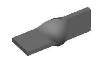
This worked nicely, thank you. A small tweak in the accuracy and
max_gradient and I have this.
Stephen
Post a reply to this message
Attachments:
Download 'smooth_twist.jpg' (5 KB)
Preview of image 'smooth_twist.jpg'

|
 |
|  |
|  |
|
 |
|
 |
|  |
|  |
|
 |
> This worked nicely, thank you. A small tweak in the accuracy and
> max_gradient and I have this.
Nice. You might even want to use this version:
#local smoothfunc = function(x) {x*x*x*(10+x*(6*x-15))}
Which also matches second derivatives, and will make the transition from
straight to curved even more invisible.
- Slime
[ http://www.slimeland.com/ ]
Post a reply to this message
|
 |
|  |
|  |
|
 |
|
 |
|  |
|  |
|
 |
Slime schrieb:
>>This worked nicely, thank you. A small tweak in the accuracy and
>>max_gradient and I have this.
>
>
> Nice. You might even want to use this version:
>
> #local smoothfunc = function(x) {x*x*x*(10+x*(6*x-15))}
>
> Which also matches second derivatives, and will make the transition from
> straight to curved even more invisible.
>
Nice, how did you calculate it?
Once I made some differential equations
for this problem and solved them.
It was a bit dirty and some paper sheets got lost.
If I remember right the differential equations
for a smooth transition from 0 to 1 were:
f(0) = 0
f(1) = 1
df(0)/dx = 0 # match in first derivative
df(1)/dx = 0
d^2f(0)/dx = 0 # match in second derivative
d^2f(1)/dx = 0
An approximation method aka Taylor or
something which could be used to get a match
in even higher derivatives would be nicer
but when I got f(x) for the second derivative
I forgot thinking about it further.
Sebastian
Post a reply to this message
|
 |
|  |
|  |
|
 |
From: Sebastian H
Subject: Re: Isosurface with straight,twist,straight
Date: 7 Mar 2005 12:37:52
Message: <422c9170@news.povray.org>
|
|
 |
|  |
|  |
|
 |
Sebastian H. schrieb:
> Slime schrieb:
>
>>> This worked nicely, thank you. A small tweak in the accuracy and
>>> max_gradient and I have this.
>>
>>
>>
>> Nice. You might even want to use this version:
>>
>> #local smoothfunc = function(x) {x*x*x*(10+x*(6*x-15))}
>>
>> Which also matches second derivatives, and will make the transition from
>> straight to curved even more invisible.
>>
>
> Nice, how did you calculate it?
> Once I made some differential equations
> for this problem and solved them.
> It was a bit dirty and some paper sheets got lost.
> If I remember right the differential equations
> for a smooth transition from 0 to 1 were:
>
> f(0) = 0
> f(1) = 1
>
> df(0)/dx = 0 # match in first derivative
> df(1)/dx = 0
>
> d^2f(0)/dx = 0 # match in second derivative
> d^2f(1)/dx = 0
>
> An approximation method aka Taylor or
> something which could be used to get a match
> in even higher derivatives would be nicer
> but when I got f(x) for the second derivative
> I forgot thinking about it further.
>
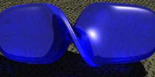
And here is my image from then.
Sebastian
Post a reply to this message
Attachments:
Download 'twist.jpg' (19 KB)
Preview of image 'twist.jpg'

|
 |
|  |
|  |
|
 |
|
 |
|  |
|  |
|
 |
> Nice, how did you calculate it?
Actually, I just took it from my old Slime-POV source code which implemented
second-derivative continuity in f_noise3d; so ultimately it came from Ken
Perlin's paper which explained how to do that. Of course, it can be figured
out manually with the conditions you describe. Since there are 6
restrictions on the function, we must have 6 unknowns, which mean it's a 5th
order equation:
f(x) = ax^5 + bx^4 + cx^3 + dx^2 + ex + f
Differentiating twice, plugging in x = 0 or 1 and setting the results equal
to zero or one as you stated should produce a 6x6 matrix which can be solved
for a,b,c,d,e,f. The result will be a=6, b=-15, c=10, d=e=f=0. Then the
result is equivalent to x*x*x*(10+x*(6*x-15)).
Nice image, the smoothness really helps.
- Slime
[ http://www.slimeland.com/ ]
Post a reply to this message
|
 |
|  |
|  |
|
 |
|
 |
|  |
|  |
|
 |
Slime schrieb:
>>Nice, how did you calculate it?
>
>
> Actually, I just took it from my old Slime-POV source code which implemented
> second-derivative continuity in f_noise3d; so ultimately it came from Ken
> Perlin's paper which explained how to do that. Of course, it can be figured
> out manually with the conditions you describe. Since there are 6
> restrictions on the function, we must have 6 unknowns, which mean it's a 5th
> order equation:
>
> f(x) = ax^5 + bx^4 + cx^3 + dx^2 + ex + f
>
> Differentiating twice, plugging in x = 0 or 1 and setting the results equal
> to zero or one as you stated should produce a 6x6 matrix which can be solved
> for a,b,c,d,e,f. The result will be a=6, b=-15, c=10, d=e=f=0. Then the
> result is equivalent to x*x*x*(10+x*(6*x-15)).
This is exactly how I did it but I kept some variables
in the matrix, therefore it got a bit messy (had nothing to do then).
> Nice image, the smoothness really helps.
Thank you.
I allways enjoy your images, too.
Sebastian
Post a reply to this message
|
 |
|  |
|  |
|
 |
|
 |
|  |
|  |
|
 |
> I allways enjoy your images, too.
Thank you!
- Slime
[ http://www.slimeland.com/ ]
Post a reply to this message
|
 |
|  |
|  |
|
 |
|
 |
|  |
|
 |


![]()