|
 |
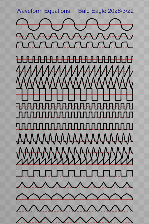
I have a small library of periodic waveforms.
Note that it's a practical library, sometimes with different ways of
implementing the same general shape.
Some could be trimmed down.
Some could be expanded by adding named parameters that control the shape.
Having differentiable curves would be useful for people who have need for, and
know what they're doing with that sort of thing.
I know that there are a lot of "smoothing functions" out there for use in
animations,
There are some nice polar equations out there.
These should all be standard tools that we can easily implement in scenes.
// Waveform Equations
// Bill "Bald Eagle" Walker 2026/3/22
#version version;
global_settings {assumed_gamma 1.0}
#declare Zoom = 20;
camera {
orthographic
location <10, 19, -50>
right x*image_width/Zoom
up y*image_height/Zoom
look_at <10, 19, 0>
}
light_source {<40, 30, -50> rgb 1 shadowless}
sky_sphere {pigment {rgb 1}}
plane {z, 0.01 pigment {checker rgb 0.9 rgb 0.8}}
#declare Axes =
union {
#declare Line = 0.05;
#declare Base = Line*2;
#declare Length = 10;
#declare Ext = 0.25;
cylinder {<0, 0, 0>, <Length, 0, 0>, Line pigment {rgb x}}
cone {<Length, 0, 0>, Base, <Length+Ext, 0, 0>, 0 pigment {rgb x} }
cylinder {<0, 0, 0>, <0, Length, 0>, Line pigment {rgb y}}
cone {<0, Length, 0>, Base, <0, Length+Ext, 0>, 0 pigment {rgb y}}
cylinder {<0, 0, 0>, <0, 0, Length>, Line pigment {rgb z}}
cone {<0, 0, Length>, Base, <0, 0, Length+Ext>, 0 pigment {rgb z}}
}
//object {Axes}
#declare E = 1e-9;
#declare Inf = 1e10;
#declare Line = 0.08;
#declare Extent = 20;
#declare Step = 0.01;
#declare even = function(N) {select(mod(N, 2), 0, 1, 0)}
#declare odd = function(N) {select(mod(N, 2), 1, 0, 1)}
#declare sgn = function(N) {select(N, -1, 0, 1)}
#declare cot = function (N) {1/tan(N)}
#declare sec = function (N) {1/cos(N)}
#declare csc = function (N) {select (sin(N), 1/sin(N), Inf, 1/sin(N))}
#declare Amplitude = 1;
#declare Period = 1;
#declare a = 1;
#declare b = 1;
#declare c = 0;
#declare f = 1;
#declare m = 1;
#declare l = 1;
#declare p = 1;
#declare T = 0.3; // how long pulse wave stays at 1
// capacitor charge-discharge
//
https://www.syncad.com/waveform_block_equations_for_timing_diagram_editors.htm
#declare pns = 0.2;
#declare pps = pns * 10;
#declare rcns = 0.01;
#declare rcps = 10 * rcns;
#declare Sample = function (N) {mod(N, pps/2)}
#declare Charge = function (N) {select (mod(floor(N/(pps/2)),2), 1, 0, 1)}
#declare Waveforms = array {
function (N) {abs(-odd(floor(N))+mod(N, 1))},
function (N) {1-(cos(N*pi)*0.5+0.5)},
function (N) {sqrt(abs(-odd(floor(N))+mod(N, 1)) )},
function (N) {pow(abs(-odd(floor(N))+mod(N, 1)), 2)},
function (N) {select (mod(N, 2)-1, 0, 1)},
function (N) {mod (N, 1)},
function (N) {(-3*pow(sin(N*3), 2)*sin(N*6))*0.5},
function (N) {-pow(sin(N*3), 2)*(a*cos(N*6) + b*sin(N*6))},
//function (N) {-cos(N*3)*(cos(N*6)+sin(N*6))},
function (N) {sgn (sin (2*pi*f*N))/2+0.5},
function (N) {-(2*floor(f*N)-floor(2*f*N))},
function (N) {pow (-1, floor(2*f*N))/2},
function (N) {(2/pi) * atan (tan (pi*f*N/2)) + (2/pi) * atan (cot (pi*f*N/2))},
function (N) {(4/p)*(N-(p/2)*floor(2*N/p+0.5))*pow(-1,floor(2*N/p+0.5))},
function (N) {2*(N/p-floor(0.5+N/p))},
function (N) {sgn (cos(2*pi*N/p)-cos(pi*T/p)) * 0.5},
function (N) {select (Charge(N), 0, a*(1-exp(-Sample(N)/rcps)),
a*exp(-Sample(N)/rcps) )},
function (N) {(a/pi) * (asin(sin((pi/m)*N+l)) + acos(cos((pi/m)*N+l))) - (a/2)
+ c},
function (N) {pow(-1, floor(N/2))*sqrt (1-pow((mod(N,2)-1),2))}
};
#declare NF = dimension_size (Waveforms, 1)-1;
#declare Abscissa = x;
#declare Ordinate = y;
// Applicate: The z-coordinate (the last of the three terms by which a point is
referred to,
// in a system of Cartesian coordinates for a three-dimensional space)
#local ZeroVector = <0, 0, 0>;
#for (F, 0, NF)
#ifdef(Function) #undef Function #end
#local Function = Waveforms [F];
//#debug concat ("F = ", str(F, 0, 0), "\n")
#local Shift_Y = y*F*2;
cylinder {<0, F*2, 0>, <Extent, F*2, 0> Line*0.75 pigment {checker rgb x rgbf 1
scale 0.25}}
union {
#for (i, 0, Extent, Step)
#local Value = Function (i);
#local A = Abscissa * i;
#local O = Ordinate * Value + Shift_Y;
#local Current = A + O + ZeroVector;
sphere {Current, Line}
#if (i > 0)
cylinder {Last, Current+E Line}
#end
#local Last = Current;
#end
pigment {rgb 0}
}
#end
text { ttf "arial.ttf", "Waveform Equations Bald Eagle 2026/3/22", 0.02, 0.0
pigment {rgb z*0.4} translate y*(F)*2}
Post a reply to this message
Attachments:
Download 'waveforms.png' (145 KB)
Preview of image 'waveforms.png'
|
|